In this article, Youssef LOURAOUI (ESSEC Business School, Global Bachelor of Business Administration, 2017-2021) presents the different alternatives developed to the market-capitalization weighting strategy (buy-and-hold strategy).
The structure of this post is as follows: we begin by introducing alternatives to market capitalization strategies as a topic. We then will delve deeper by presenting heuristic-based weighting and optimization-based weighting strategies.
Introduction
The basic rule of applying a market-capitalization weighting methodology for the development of indexes has recently come under fire. As the demand for indices as investment vehicles has grown, different weighting systems have emerged. There have also been a number of recent projects for non-market-capitalization-weighted ETFs. Since the first basic factor weighted ETF was released in May 2000, a slew of ETFs has been released to monitor non-market-cap-weighted indexes, including equal-weighted ETFs, minimal variance ETFs, characteristics-weighted ETFs, and so on. These are dubbed “Smart Beta ETFs” since they aim to outperform traditional market-capitalization-based indexes in terms of risk-adjusted returns (Amenc et al. 2016).
The categorization approach will be the same as Chow, Hsu, Kalesnik, and Little (2011), with the following distinctions: 1) basic weighting techniques (heuristic-based weighting) and 2) more advanced quantitative weighting techniques (optimization-based weighting).
It’s an arbitrary categorization system designed to make reading easier by differentiating between simpler and more complicated approaches.
Heuristic-based weighting strategies
Equal-weighting
The equal weighting method assigns the same weight to each share making up the portfolio (or index)

Where wi represents the weight of asset i in the portfolio and N the total number of assets in the portfolio.
Because each component of the portfolio has the same weight, equal weighting helps investors to obtain more exposure to smaller firms. Bigger firms will be more represented in the market-capitalization-weighted portfolio since their weight will be larger. The benefit of this technique is that tiny capitalization risk-adjusted-performance tends to be better than big capitalization (Banz, 1981).
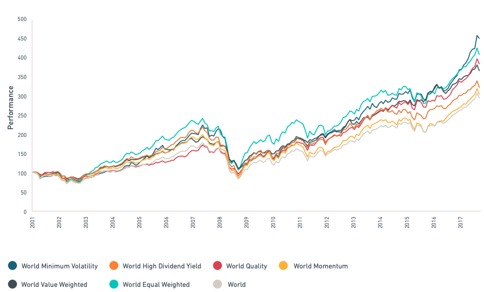
In their study, Arnott, Kalesnik, Moghtader, and Scholl (2010) created three distinct indices in terms of index composition. The first group consists of enterprises with substantial market capitalization (as are capitalisation-weighted indices). Each business in the index is then given equal weight. This is how the majority of equally-weighted indexes are built (MSCI World Equal Index, S&P500 Equal Weight Index). The second is to create an index based on basic criteria and then assign equal weight to each firm. The third strategy is a hybrid of the first two. It entails averaging the ranks from the two preceding approaches and then assigning equal weight to the remaining 1000 shares.
Fundamental-weighting
The weighting approach based on fundamentals divides companies into categories based on their basic size. Sales, cash flow, book value, and dividends are all taken into account. These four parameters are used to determine the top 1,000 firms, and each firm in the index is given a weight based on the magnitude of their individual components (Arnott et al., 2005). The portfolio weight of the ith stock is defined as:
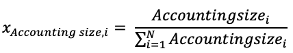
For a fundamental index that includes book value as a consideration, for example, the top 1,000 companies in the market with the most extensive book values are chosen. Firm xi is given a weight wi, which is equal to the firm’s book value divided by the total of the index components’ book values.
Fundamental indexation tries to address the following bias: in a cap-weighted index, if the market efficiency hypothesis is not validated and a share’s price is, for example, overpriced (greater than its fair value), the share’s weight in the index will be too high. Weighting by fundamentals will reduce the bias of over/underweighting over/undervalued companies based on criteria like sales, cash flows, book value, and dividends, which are not affected by market opinion, unlike capitalization.
Low beta weighting
Low-beta strategies are based on the fact that equities with a low beta have greater returns than those expected by the CAPM (Haugen and Heins, 1975). A beta of less than one indicates that the share price has tended to grow less than its benchmark index during bullish trends and to decrease less severely during negative trends throughout the observed timeframe. A low-beta index is created by selecting low-beta stocks and then giving each stock equal weight in the index. As a result, it’s a hybrid of a low-beta and an equal-weighting method. On the other side, high beta strategies enable investors to profit from the amplification of favourable market moves.
Reverse-capitalization weighting
The weight of an asset capitalization-weighted index can be defined as:
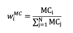
where MC stands for “Market Capitalization”, and wi is the weight of asset i in the portfolio.
In a reverse market-capitalization-weighted index, the weight of an asset is defined as:
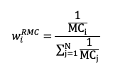
“Reverse market-capitalization” is abbreviated as RMC. This technique necessitates using a cap-weighted index to execute the approach. RCW methods, like equal-weight or low-beta strategies, are motivated by the fact that small caps have a greater risk-adjusted return than big caps. This sort of indexation requires constant rebalancing (Banz, 1981).
Maximum diversification
This technique aims to build a portfolio with as much diversification as feasible. A diversity index (DI) is employed to achieve the desired outcome, which is defined as the distance between the sum of the constituents’ volatilities and the portfolio’s volatility (Amenc, Goltz, and Martellini, 2013). Diversity weighting is one of the better-known portfolio heuristics that blend cap weighting and equal weighting. Fernholz (1995) defined stock market diversity, Dp, as
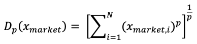
where p between (0,1) and x Market,i is the weight of the ith stock in the cap-weighted market portfolio, and then proposed a strategy of portfolio weighting whereby portfolio weights are defined as
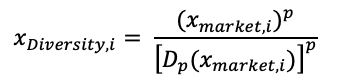
where i = 1, . . . , N; p between (0,1); and the parameter p targets the desired level of portfolio tracking error against the cap-weighted index.
Optimization-based weighting strategies
The logic of Modern Portfolio Theory (Markowitz, 1952) is followed in Mean-Variance optimization. Theoretically, if we know the expected returns of all stocks and their variance-covariance matrix, we can construct risk-adjusted-performance optimal portfolios. However, these two inputs for the model are difficult to estimate precisely in practice. Chopra and Ziemba (1993) showed that even little inaccuracies in these parameters’ estimates may have a large influence on risk-adjusted-performance.
Minimum Variance
Chopra and Ziemba (1993) adopt the simple premise that all stocks have the same return expectation, based on the fact that stock return expectations are difficult to quantify. As a result of this premise, the best portfolio is the one that minimizes risk. The goal of minimal variance strategies, which have been around since 1990, is to provide a better risk-return profile by lowering portfolio risk without modifying return expectations. The low volatility anomaly justifies this technique. Low-volatility stocks have historically outperformed high-volatility equities. These portfolios are built without using a benchmark as a guide. The portfolio variance minimization equation for a two-asset portfolio is as follows:

In their research on the construction of this type of index, Arnott, Kalesnik, Moghtader and Scholl (2010) found that risk measures that take into account interest rates, oil prices, geographical region, sector, size, expected return, and growth, as calculated by the Northfield global risk model, a model for making one-year risk forecasts, reduce the portfolio’s absolute risk. This method is used in the MSCI World Minimum Volatility Index, which was released in 2008.
Global Minimum Variance, Maximum Decorrelation, and Diversified Minimum Variance are the three types of minimum variance techniques (Amenc, Goltz and Martellini, 2013). However, there are no indexes or exchange-traded funds (ETFs) based on the Maximum Decorrelation and Diversified Minimum Variance methods in actuality; they are still only theoretical notions.
Maximum Sharpe ratio
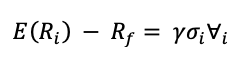
Because all stocks are unlikely to have the same expected returns, the minimum-variance portfolio—or any practical representation of its concept—is unlikely to have the highest ex-ante Sharpe ratio. Investors must incorporate useful information about future stock returns into a minimum-variance approach to improve it. Choueifaty and Coignard (2008) proposed a simple linear relationship between the expected premium, E(Ri) – Rf, for a stock and its return volatility, sigmai:
A related portfolio method proposed by Amenc, Goltz, Martellini, and Retkowsky (2010) implies that a stock’s expected returns are linearly related to its downside semi-volatility. They claimed that portfolio losses are more important to investors than gains. As a result, rather than volatility, risk premium should be connected to downside risk (semi-deviation below zero). The EDHEC-Risk Efficient Equity Indices are built around this assumption. Downside semi-volatility can be defined mathematically as
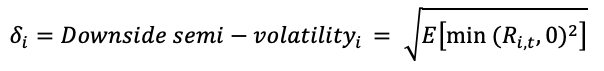
where Ri, t is the return for stock i in period t.
Maximum Sharpe ratio can be considered as an alternative beta technique that aims to solve the challenges of forecasting risks and returns for a large number of equities.
Why should I be interested in this post?
If you are a business school or university undergraduate or graduate student, this content will help you in understanding the various evolutions of asset management throughout the last decades and in broadening your knowledge of finance.
Smart beta funds have become a hot issue among investors in recent years. Smart beta is a game-changing invention that addresses an unmet need among investors: a higher return for lower risk, net of transaction and administrative costs. In a way, these investment strategies create a new market. As a result, smart beta is gaining traction and influencing the asset management industry.
Related posts on the SimTrade blog
Factor investing
▶ Youssef LOURAOUI Factor Investing
▶ Youssef LOURAOUI Origin of factor investing
▶ Youssef LOURAOUI Smart beta 1.0
▶ Youssef LOURAOUI Smart beta 2.0
Factors
▶ Youssef LOURAOUI Size Factor
▶ Youssef LOURAOUI Value Factor
▶ Youssef LOURAOUI Yield Factor
▶ Youssef LOURAOUI Momentum Factor
▶ Youssef LOURAOUI Quality Factor
▶ Youssef LOURAOUI Growth Factor
▶ Youssef LOURAOUI Minimum Volatility Factor
Useful resources
Academic research
Amenc, Noël, Felix Goltz, Lionel Martellini, and Patrice Ret- kowsky. 2010. “Efficient Indexation: An Alternative to Cap- Weighted Indices.” EDHEC-Risk Institute (February).
Amenc, N., Goltz, F., Le Sourd, V., 2016. Investor perception about Smart beta ETF. EDHEC Risk Institute working paper.
Amenc, N., Goltz, F., Martinelli, L., 2013. Smart beta 2.0. EDHEC Risk Institute working paper.
Arnot, R.D., Hsu, J., Moore, P., 2005. Fundamental Indexation. Financial Analysts Journal, 61(2):83-98.
Arnot, R.D., Kalesnik, V., Moghtader, P., Scholl, S., 2010. Beyond Cap Weight, The empirical evidence for a diversified beta. Journal of Indexes, January, 16-29.
Banz, R., 1981. The relationship between return and market value of common stocks. Journal of Financial Economics. 9(1):3-18.
Chopra, V., Ziemba, W., 1993. The Effect of Errors in Means, Variances, and Covariances on Optimal Portfolio Choice. Journal of Portfolio Management, 19:6-11.
Chow, T., Hsu, J., Kalesnik, V., Little, B., 2011. A Survey of Alternative Equity Index Strategies. Financial Analyst Journal, 67(5):35-57.
Choueifaty, Yves, and Yves Coignard. 2008. Toward Maximum Diversification. Journal of Portfolio Management, vol. 35, no. 1 (Fall):40–51.
Fernholz, Robert. 1995. Portfolio Generating Functions. Working paper, INTECH (December).
Haugen, R., Heins, J., 1975. Risk and Rate of Return of Financial Assets: Some Old Wine in New Bottles. Journal of Financial and Quantitative Analysis, 10(5):775-784.
Markowitz, H., 1952. Portfolio Selection. The Journal of Finance, 7(1):77-91.
About the author
The article was written in September 2021 by Youssef LOURAOUI (ESSEC Business School, Global Bachelor of Business Administration, 2017-2021).