Copula

In this article, Shengyu ZHENG (ESSEC Business School, Grande Ecole Program – Master in Management, 2020-2024) presents copula, a statistical tool that is commonly used to model dependency of random variables.

Linear correlation

In the world stacked with various risks, a simplistic look of individual risks does not suffice, since the interactions between risks could add to or diminish the aggregate risk loading. As we often see in statistical modelling, linear correlation, as one of the simplest ways to look at dependency between random variables, is commonly used for this purpose.

Definition of linear correlation

To put it concisely, the linear correlation coefficient, denoted by ‘ρ(X,Y)’, takes values within the range of -1 to 1 and represents the linear correlation of two random variables X and Y. A positive ‘ρ(X,Y)’ indicates a positive linear relationship, signifying that as one variable increases, the other tends to increase as well. Conversely, a negative ‘ρ(X,Y)’ denotes a negative linear relationship, signifying that as one variable increases, the other tends to decrease. A correlation coefficient near zero implies a lack of linear relation.

Limitation of linear correlation

As a simplistic model, while having the advantage of easy application, linear correlation fails to capture the intricacy of the dependance structure between random variables. There exist three main limitations of linear correlation.

• ρ(X,Y) only gives a scalar summary of linear dependence and it requires that both var(X) and var(Y) must exist and finite;
• Given that assumption that X and Y are stochastically independent, it can be inferred that ρ(X,Y) = 0. Whereas, the converse does not stand for most of the cases (except if (X,Y) is a Gaussian random vector).
• Linear correlation is not invariant with regard to strict increasing transformations. If T is such a transformation, ρ(T(X),T(Y)) ≠ ρ(X,Y)

Therefore, if we have in hand the marginal distributions of two random variables and their linear correlations, it does not suffice to determine the joint distribution.

Copula

A copula is a mathematical function that describes the dependence structure between multiple random variables, irrespective of their marginal distributions. It describes the interdependency that transcends linear relationships. Copulas are employed to model the joint distribution of variables by separating the marginal distributions from the dependence structure, allowing for a more flexible and comprehensive analysis of multivariate data. Essentially, copulas serve as a bridge between the individual distributions of variables and their joint distribution, enabling the characterization of their interdependence.

Definition of copula

A copula, denoted typically as C∶[0,1]^d→[0,1] , is a multivariate distribution function whose marginals are uniformly distributed on the unit interval. The parameter d is the number of variables. For a set of random variables U₁, …, U_d with cumulative distribution functions F₁, …, F_d, the copula function C satisfies:

C(F₁(u₁),…,F_d(u_d)) = ℙ(U₁≤u₁,…,U_d≤u_d)

Fréchet-Hoeffding bounds

The Fréchet–Hoeffding theorem states that copulas follow the bounds:

max{1 – d + ∑^d_i=1u_i} ≤ C(u) ≤ min{u₁, …, u_d}

In a bivariate case (dimension equals 2), the Fréchet–Hoeffding bounds are

max{u+v-1,0} ≤ C(u,v) ≤ min{u,v}

The upper bound corresponds to the case of comonotonicity (perfect positive dependence) and the lower bound corresponds to the case of countermonotonicity (perfect negative dependence).

Sklar’s theorem

Sklar’s theorem states that every multivariate cumulative distribution function of a random vector X can be expressed in terms of its marginals and a copula. The copula is unique if the marginal distributions are continuous. The theorem states also that the converse is true.

Sklar’s theorem shows how a unique copula C fully describes the dependence of X. The theorem provides a way to decompose a multivariate joint distribution function into its marginal distributions and a copula function.

Examples of copulas

Many types of dependence structures exist, and new copulas are being introduced by researchers. There are three standard classes of copulas that are commonly in use among practitioners: elliptical or normal copulas, Archimedean copulas, and extreme value copulas.

Elliptical or normal copulas

The Gaussian copula and the Student-t copula are among this category. Be reminded that the Gaussian copula played a notable role in the 2008 financial crisis, particularly in the context of mortgage-backed securities and collateralized debt obligations (CDOs). The assumption of normality and underestimation of systemic risk based on the Gaussian copula failed to account for the extreme risks in face of crisis.

Here is an example of a simulated normal copula with the parameter being 0.8.

Figure 1. Simulation of normal copula.

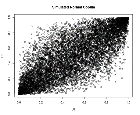
Source: computation by the author.

Archimedean copulas

Archimedean copulas are a class of copulas that have a particular mathematical structure based on Archimedean copula families. These copulas have a connection with certain mathematical functions known as Archimedean generators.

Here is an example of a simulated Clayton copula with the parameter being 3, which is from the category of Archimedean copulas

Figure 2. Simulation of Clayton copula.

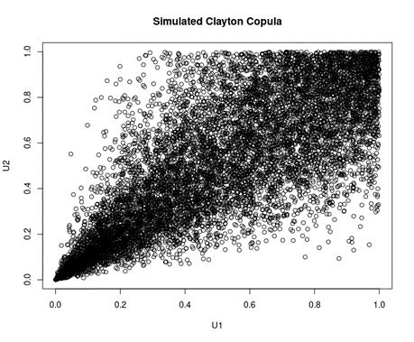
Source: computation by the author.

Extreme value copulas

Extreme value copulas could overlap with the two other classes. They are a specialized class of copulas designed to model the tail dependence structure of multivariate extreme events. These copulas are particularly useful in situations where the focus is on capturing dependencies in the extreme upper or lower tails of the distribution.

Here is an example of a simulated Tawn copula with the parameter being 0.8, which is from the category of extreme value copulas

Figure 3. Simulation of Tawn copula.

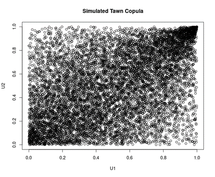
Source: computation by the author.

Download R file to simulate copulas

You can find below an R file (file with txt format) to simulate the 3 copulas mentioned above.

Why should I be interested in this post?

Copulas are pivotal in risk management, offering a sophisticated approach to model the dependence among various risk factors. They play a crucial role in portfolio risk assessment, providing insights into how different assets behave together and enhancing the robustness of risk measures, especially in capturing tail dependencies. Copulas are also valuable in credit risk management, aiding in the assessment of joint default probabilities and contributing to an understanding of credit risks associated with diverse financial instruments. Their applications extend to insurance, operational risk management, and stress testing scenarios, providing a toolset for comprehensive risk evaluation and informed decision-making in dynamic financial environments.

Related posts on the SimTrade blog

▶ Shengyu ZHENG Moments de la distribution

▶ Shengyu ZHENG Mesures de risques

▶ Shengyu ZHENG Extreme Value Theory: the Block-Maxima approach and the Peak-Over-Threshold approach

▶ Gabriel FILJA Application de la théorie des valeurs extrêmes en finance de marchés

Useful resources

Course notes from Quantitative Risk Management of Prof. Marie Kratz, ESSEC Business School.

About the author

The article was written in November 2023 by Shengyu ZHENG (ESSEC Business School, Grande Ecole Program – Master in Management, 2020-2024).