Portfolio Archives

Hedge fund diversification

January 13, 2023 by Youssef LOURAOUI

In this article, Youssef LOURAOUI (Bayes Business School, MSc. Energy, Trade & Finance, 2021-2022) discusses the notion of hedge fund diversification by analyzing the paper “Hedge fund diversification: how much is enough?” by Lhabitant and Learned (2002).

This article is organized as follows: we describe the primary characteristics of the research paper. Then, we highlight the research paper’s most important points. This essay concludes with a discussion of the principal findings.

Introduction

The paper discusses the advantages of investing in a set of hedge funds or a multi-strategy hedge fund. It is a relevant subject in the field of alternative investments since it has attracted the interest of institutional investors seeking to uncover the alternative investment universe and increase their portfolio return. The paper’s primary objective is to determine the appropriate number of hedge funds that an portfolio manager should combine in its portfolio to maximise its (expected) returns. The purpose of the paper is to examine the impact of adding hedge funds to a traditional portfolio and its effect on the various statistics (average return, volatility, skewness, and kurtosis). The authors consider basic portfolios (randomly chosen and equally-weighted portfolios). The purpose is to evaluate the diversification advantage and the dynamics of the diversification effect of hedge funds.

Key elements of the paper

The pioneering work of Henry Markowitz (1952) depicted the effect of diversification by analyzing the portfolio asset allocation in terms of risk and (expected) return. Since unsystematic risk (specific risk) can be neutralized, investors will not receive an additional return. Systematic risk (market risk) is the component that the market rewards. Diversification is then at the heart of asset allocation as emphasized by Modern Portfolio Theory (MPT). The academic literature has since then delved deeper on the analysis of the optimal number of assets to hold in a well-diversified portfolio. We list below some notable contributions worth mentioning:

Elton and Gruber (1977), Evans and Archer (1968), Tole (1982) and Statman (1987) among others delved deeper into the optimal number of assets to hold to generate the best risk and return portfolio. There is no consensus on the optimal number of assets to select.
Evans and Archer (1968) depicted that the best results are achieved with 8-10 assets, while raising doubts about portfolios with number of assets above the threshold. Statman (1987) concluded that at least thirty to forty stocks should be included in a portfolio to achieve the portfolio diversification.

Lhabitant and Learned (2002) also mention the concept of naive diversification (also known as “1/N heuristics”) is an allocation strategy where the investor split the overall fund available is distributed into same. Naive diversification seeks to spread asset risk evenly in the portfolio to reduce overall risk. However, the authors mention important considerations for naïve/Markowitz optimization:

Drawback of naive diversification: since it doesn’t account for correlation between assets, the allocation will yield a sub-optimal result and the diversification won’t be fully achieved. In practice, naive diversification can result in portfolio allocations that lie on the efficient frontier. On the other hand, mean-variance optimisation, the framework revolving he Modern Portfolio Theory is subject to input sensitivity of the parameters used in the optimization process. On a side note, it is worth mentioning that naive diversification is a good starting point, better than gut feeling. It simplifies allocation process while also benefiting by some degree of risk diversification.
Non-normality of distribution of returns: hedge funds exhibit non-normal returns (fat tails and skewness). Those higher statistical moments are important for investors allocation but are disregarded in a mean-variance framework.
Econometric difficulties arising from hedge fund data in an optimizer framework. Mean-variance optimisers tend to consider historical return and risk, covariances as an acceptable point to assess future portfolio performance. Applied in a construction of a hedge fund portfolio, it becomes even more difficult to derive the expected return, correlation, and standard deviation for each fund since data is scarcer and more difficult to obtain. Add to that the instability of the hedge funds returns and the non-linearity of some strategies which complicates the evaluation of a hedge fund portfolio.
Operational risk arising from fund selection and implementation of the constraints in an optimiser software. Since some parameters are qualitative (i.e., lock up period, minimum investment period), these optimisers tool find it hard to incorporate these types of constraints in the model.

Conclusion

Due to entry restrictions, data scarcity, and a lack of meaningful benchmarks, hedge fund investing is difficult. The paper analyses in greater depth the optimal number of hedge funds to include in a diversified portfolio. According to the authors, adding funds naively to a portfolio tends to lower overall standard deviation and downside risk. In this context, diversification should be improved if the marginal benefit of adding a new asset to a portfolio exceeds its marginal cost.

The authors reiterate that investors should not invest “naively” in hedge funds due to their inherent risk. The impact of naive diversification on the portfolio’s skewness, kurtosis, and overall correlation structure can be significant. Hedge fund portfolios should account for this complexity and examine the effect of adding a hedge fund to a well-balanced portfolio, taking into account higher statistical moments to capture the allocation’s impact on portfolio construction. Naive diversification is subject to the selection bias. In the 1990s, the most appealing hedge fund strategy was global macro, although the long/short equity strategy acquired popularity in the late 1990s. This would imply that allocations will be tilted towards these two strategies overall.

The answer to the title of the research paper? Hedge funds portfolios should hold between 15 and 40 underlying funds, while most diversification benefits are reached when accounting with 5 to 10 hedge funds in the portfolio.

Why should I be interested in this post?

The purpose of portfolio management is to maximise returns on the entire portfolio, not just on one or two stocks. By monitoring and maintaining your investment portfolio, you can accumulate a substantial amount of wealth for a range of financial goals, such as retirement planning. This article facilitates comprehension of the fundamentals underlying portfolio construction and investing. Understanding the risk/return profiles, trading strategy, and how to incorporate hedge fund strategies into a diversified portfolio can be of great interest to investors.

Useful resources

Academic research

Elton, E., and M. Gruber (1977). “Risk Reduction and Portfolio Size: An Analytical Solution.” Journal of Business, 50. pp. 415-437.

Evans, J.L., and S.H. Archer (1968). “Diversification and the Reduction of Dispersion: An Empirical Analysis”. Journal of Finance, 23. pp. 761-767.

Lhabitant, François S., Learned Mitchelle (2002). “Hedge fund diversification: how much is enough?” Journal of Alternative Investments. pp. 23-49.

Markowitz, H.M (1952). “Portfolio Selection.” The Journal of Finance, 7, pp. 77-91.

Statman, M. (1987). “How many stocks make a diversified portfolio?”, Journal of Financial and Quantitative Analysis , pp. 353-363.

Tole T. (1982). “You can’t diversify without diversifying”, Journal of Portfolio Management, 8, pp. 5-11.

About the author

The article was written in January 2023 by Youssef LOURAOUI (Bayes Business School, MSc. Energy, Trade & Finance, 2021-2022).

Minimum Volatility Portfolio

January 9, 2023 by Youssef LOURAOUI

In this article, Youssef LOURAOUI (Bayes Business School, MSc. Energy, Trade & Finance, 2021-2022) elaborates on the concept of Minimum Volatility Portfolio, which is derived from Modern Portfolio Theory (MPT) and also in practice to build investment funds.

This article is structured as follows: we introduce the concept of Minimum Volatility Portfolio. Next, we present some interesting academic findings, and we finish by presenting a theoretical example to support the explanations given in this article.

Introduction

The minimum volatility portfolio represents a portfolio of assets with the lowest possible risk for an investor and is located on the far-left side of the efficient frontier. Note that the minimum volatility portfolio is also called the minimum variance portfolio or more precisely the global minimum volatility portfolio (to distinguish it from other optimal portfolios obtained for higher risk levels).

Modern Portfolio Theory’s fundamental notion had significant implications for portfolio construction and asset allocation techniques. In the late 1970s, the portfolio management business attempted to capture the market portfolio return. However, as financial research progressed and some substantial contributions were made, new factor characteristics emerged to capture extra performance. The financial literature has long encouraged taking on more risk to earn a higher return. However, this is a common misconception among investors. While extremely volatile stocks can produce spectacular gains, academic research has repeatedly proved that low-volatility companies provide greater risk-adjusted returns over time. This occurrence is known as the “low volatility anomaly,” and it is for this reason that many long-term investors include low volatility factor strategies in their portfolios. This strategy is consistent with Henry Markowitz’s renowned 1952 article, in which he embraces the merits of asset diversification to form a portfolio with the maximum risk-adjusted return.

Academic Literature

Markowitz is widely regarded as a pioneer in financial economics and finance due to the theoretical implications and practical applications of his work in financial markets. Markowitz received the Nobel Prize in 1990 for his contributions to these fields, which he outlined in his 1952 Journal of Finance article titled “Portfolio Selection.” His seminal work paved the way for what is now commonly known as “Modern Portfolio Theory” (MPT).

In 1952, Harry Markowitz created modern portfolio theory with his work. Overall, the risk component of MPT may be evaluated using multiple mathematical formulations and managed through the notion of diversification, which requires building a portfolio of assets that exhibits the lowest level of risk for a given level of expected return (or equivalently a portfolio of assets that exhibits the highest level of expected return for a given level of risk). Such portfolios are called efficient portfolios. In order to construct optimal portfolios, the theory makes a number of fundamental assumptions regarding the asset selection behavior of individuals. These are the assumptions (Markowitz, 1952):

The only two elements that influence an investor’s decision are the expected rate of return and the variance. (In other words, investors use Markowitz’s two-parameter model to make decisions.) .
Investors are risk averse. (That is, when faced with two investments with the same expected return but two different risks, investors will favor the one with the lower risk.)
All investors strive to maximize expected return at a given level of risk.
All investors have the same expectations regarding the expected return, variance, and covariances for all hazardous assets. This assumption is known as the homogenous expectations assumption.
All investors have a one-period investment horizon.

Only in theory does the minimum volatility portfolio (MVP) exist. In practice, the MVP can only be estimated retrospectively (ex post) for a particular sample size and return frequency. This means that several minimum volatility portfolios exist, each with the goal of minimizing and reducing future volatility (ex ante). The majority of minimum volatility portfolios have large average exposures to low volatility and low beta stocks (Robeco, 2010).

Example

To illustrate the concept of the minimum volatility portfolio, we consider an investment universe composed of three assets with the following characteristics (expected return, volatility and correlation):

Asset 1: Expected return of 10% and volatility of 10%
Asset 2: Expected return of 15% and volatility of 20%
Asset 3: Expected return of 22% and volatility of 35%

Correlation between Asset 1 and Asset 2: 0.30
Correlation between Asset 1 and Asset 3: 0.80
Correlation between Asset 2 and Asset 3: 0.50

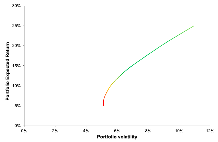
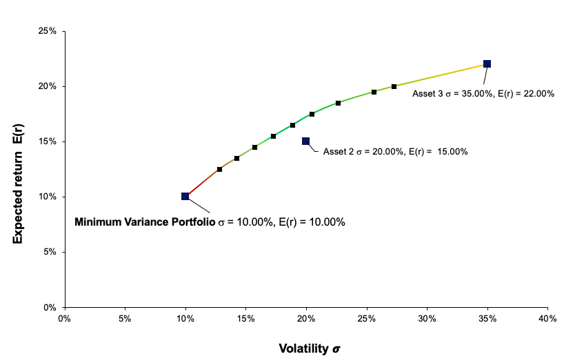
The first step to achieve the minimum variance portfolio is to construct the portfolio efficient frontier. This curve represents all the portfolios that are optimal in the mean-variance sense. After solving the optimization program, we obtain the weights of the optimal portfolios. Figure 1 plots the efficient frontier obtained from this example. As captured by the plot, we can see that the minimum variance portfolio in this three-asset universe is basically concentrated on one holding (100% on Asset 1). In this instance, an investor who wishes to minimize portfolio risk would allocate 100% on Asset 1 since it has the lowest volatility out of the three assets retained in this analysis. The investor would earn an expected return of 10% for a volatility of 10% annualized (Figure 1).

Figure 1. Minimum Volatility Portfolio (MVP) and the Efficient Frontier.

Source: computation by the author.

Excel file to build the Minimum Volatility Portfolio

You can download below an Excel file in order to build the Minimum Volatility portfolio.

Why should I be interested in this post?

Portfolio management’s objective is to optimize the returns on the entire portfolio, not just on one or two stocks. By monitoring and maintaining your investment portfolio, you can accumulate a sizable capital to fulfil a variety of financial objectives, including retirement planning. This article helps to understand the grounding fundamentals behind portfolio construction and investing.

Useful resources

Academic research

Lintner, John. 1965a. Security Prices, Risk, and Maximal Gains from Diversification. Journal of Finance, 20, 587-616.

Lintner, John. 1965b. The Valuation of Risk Assets and the Selection of Risky Investments in Stock Portfolios and Capital Budgets.Review of Economics and Statistics 47, 13-37.

Markowitz, H., 1952. Portfolio Selection. The Journal of Finance, 7, 77-91.

Sharpe, William F. 1963. A Simplified Model for Portfolio Analysis. Management Science, 19, 425-442.

Sharpe, William F. 1964. Capital Asset Prices: A Theory of Market Equilibrium under Conditions of Risk. Journal of Finance, 19, 425-442.

Business analysis

Robeco, 2010 Ten things you should know about minimum volatility investing.

About the author

The article was written in January 2023 by Youssef LOURAOUI (Bayes Business School, MSc. Energy, Trade & Finance, 2021-2022).

Optimal portfolio

December 19, 2022 by Youssef LOURAOUI

In this article, Youssef LOURAOUI (Bayes Business School, MSc. Energy, Trade & Finance, 2021-2022) presents the concept of optimal portfolio, which is central in portfolio management.

This article is structured as follows: we first define the notion of an optimal portfolio (in the mean-variance framework) and we then illustrate the concept of optimal portfolio with an example.

Introduction

An investor’s investment portfolio is a collection of assets that he or she possesses. Individual assets such as bonds and equities can be used, as can asset baskets such as mutual funds or exchange-traded funds (ETFs). When constructing a portfolio, investors typically evaluate the expected return as well as the risk. A well-balanced portfolio contains a diverse variety of investments.

An optimal portfolio is a collection of assets that maximizes the trade-off between expected return and risk: the portfolio with the highest expected return for a given level of risk, or the portfolio with the lowest risk for a given level of expected return.

To obtain the optimal portfolio, Markowitz sought to optimize the following dual program:

The first optimization seeks to maximize expected return with respect to a specific level of risk, subject to the short-selling constraint (weights of the portfolio should be equal to one).

img_SimTrade_implementing_Markowitz_2

The second optimization seeks to minimize the variance of the portfolio with respect to a specific level of expected return, subject to the short-selling constraint (weights of the portfolio should be equal to one).

img_SimTrade_implementing_Markowitz

Mathematical foundations

The investment universe is composed of N assets characterized by their expected returns μ and variance-covariance matrix V. For a given level of expected return μ_P, the Markowitz model gives the composition of the optimal portfolio. The vector of weights of the optimal portfolio is given by the following formula:

With the following notations:

w_P = vector of asset weights of the portfolio
μ_P = desired level of expected return
e = identity vector
μ = vector of expected returns
V = variance-covariance matrix of returns
V^-1 = inverse of the variance-covariance matrix
t = transpose operation for vectors and matrices

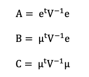
A, B and C are intermediate parameters computed below:

img_SimTrade_implementing_Markowitz_2

The variance of the optimal portfolio is computed as follows

img_SimTrade_implementing_Markowitz_3

To calculate the standard deviation of the optimal portfolio, we take the square root of the variance.

Optimal portfolio application: the case of two assets

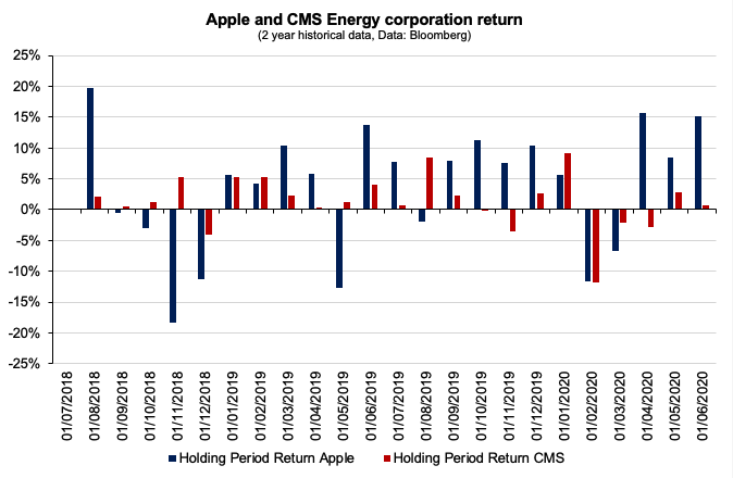
To create the optimal portfolio, we first obtain monthly historical data for the last two years from Bloomberg for two stocks that will comprise our portfolio: Apple and CMS Energy Corporation. Apple is in the technology area, but CMS Energy Corporation is an American company that is entirely in the energy sector. Apple’s historical return for the two years covered was 41.86%, with a volatility of 35.11%. Meanwhile, CMS Energy Corporation’s historical return was 13.95% with a far lower volatility of 15.16%.

According to their risk and return profiles, Apple is an aggressive stock pick in our example, but CMS Energy is a much more defensive stock that would serve as a hedge in our example. The correlation between the two stocks is 0.19, indicating that they move in the same direction. In this example, we will consider the market portfolio, defined as a theoretical portfolio that reflects the return of the whole investment universe, which is captured by the wide US equities index (S&P500 index).

As captured in Figure 1, CMS Energy suffered less severe losses than Apple. When compared to the red bars, the blue bars are far more volatile and sharp in terms of the size of the move in both directions.

Figure 1. Apple and CMS Energy Corporation return breakdown.
Time-series regression
Source: computation by the author (Data: Bloomberg)

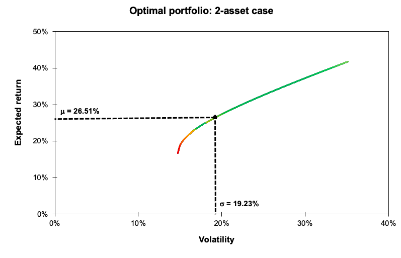
After analyzing the historical return on both stocks, as well as their volatility and covariance (and correlation), we can use Mean-Variance portfolio optimization to find the optimal portfolio. According to Markowitz’ foundational study on portfolio construction, the optimal portfolio will attempt to achieve the best risk-return trade-off for an investor. After doing the computations, we discover that the optimal portfolio is composed of 45% Apple stock and 55% CMS Energy corporation stock. This portfolio would return 26.51% with a volatility of 19.23%. As captured in Figure 2, the optimal portfolio is higher on the efficient frontier line and has a higher Sharpe ratio (1.27 vs 1.23 for the theoretical market portfolio).

Figure 2. Optimal portfolio.
Optimal portfolio plot 2 asset
Source: computation by the author (Data: Bloomberg)

You can find below the Excel spreadsheet that complements the example above.

Optimal portfolio application: the general case

We generated a large time series to obtain useful results by downloading the equivalent of 23 years of market data from a data provider (in this example, Bloomberg). We generate the variance-covariance matrix after obtaining all necessary statistical data, which includes the expected return and volatility indicated by the standard deviation of the returns for each stock during the provided period. Table 1 depicts the expected return and volatility for each stock retained in this analysis.

Table 1. Asset characteristics of Apple, Amazon, Microsoft, Goldman Sachs, and Pfizer.
img_SimTrade_implementing_Markowitz_spreadsheet_1
Source: computation by the author.

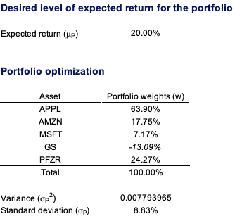
We can start the optimization task by setting a desirable expected return after computing the expected return, volatility, and the variance-covariance matrix of expected return. With the data that is fed into the appropriate cells, the model will complete the optimization task. For a 20% desired expected return, we get the following results (Table 2).

Table 2. Asset weights for an optimal portfolio.
Optimal portfolio case 1
Source: computation by the author.

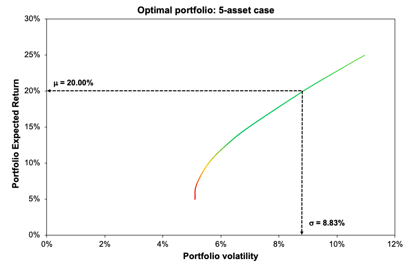
To demonstrate the effect of diversification in the reduction of volatility, we can form a Markowitz efficient frontier by tilting the desired anticipated return with their relative volatility in a graph. The Markowitz efficient frontier is depicted in Figure 1 for various levels of expected return. We highlighted the portfolio with 20% expected return with its respective volatility in the plot (Figure 3).

Figure 3. Optimal portfolio plot for 5 asset case.
Optimal portfolio case 1
Source: computation by the author.

You can download the Excel file below to use the Markowitz portfolio allocation model.

Why should I be interested in this post?

The purpose of portfolio management is to maximize the (expected) returns on the entire portfolio, not just on one or two stocks. By monitoring and maintaining your investment portfolio, you can build a substantial amount of wealth for a variety of financial goals such as retirement planning. This post facilitates comprehension of the fundamentals underlying portfolio construction and investing.

Useful resources

Academic research

Pamela, D. and Fabozzi, F., 2010. The Basics of Finance: An Introduction to Financial Markets, Business Finance, and Portfolio Management. John Wiley and Sons Edition.

Markowitz, H., 1952. Portfolio Selection. The Journal of Finance, 7(1): 77-91.

About the author

The article was written in December 2022 by Youssef LOURAOUI (Bayes Business School, MSc. Energy, Trade & Finance, 2021-2022).

Specific risk

April 1, 2022 by Youssef LOURAOUI

In this article, Youssef LOURAOUI (Bayes Business School, MSc. Energy, Trade & Finance, 2021-2022) explains the specific risk of financial assets, a key concept in asset pricing models and asset management in practice.

This article is structured as follows: we start with a reminder of portfolio theory and the central concept of risk in financial markets. We then introduce the concept of specific risk of an individual asset and especially its sources. We then detail the mathematical foundation of risk. We finish with an insight of the relationship between diversification and risk reduction with a practical example to test this concept.

Portfolio Theory and Risk

Markowitz (1952) and Sharpe (1964) created a framework for risk analysis based on their seminal contributions to portfolio theory and capital market theory. All rational profit-maximizing investors attempt to accumulate a diversified portfolio of risky assets and borrow or lend to achieve a risk level consistent with their risk preferences given a set of assumptions. They established that the key risk indicator for an individual asset in these circumstances is its correlation with the market portfolio (the beta).

The variance of returns of an individual asset can be decomposed as the sum of systematic risk and specific risk. Systematic risk refers to the proportion of the asset return variance that can be attributed to the variability of the whole market. Specific risk refers to the proportion of the asset return variance that is unconnected to the market and reflects the unique nature of the asset. Specific risk is often regarded as insignificant or irrelevant because it can be eliminated in a well-diversified portfolio.

Sources of specific risk

Specific risk can find its origin in business risk (in the assets side of the balance sheet) and financial risk (in the liabilities side of the balance sheet):

Business risk

Internal or external issues might jeopardize a business. Internal risk is directly proportional to a business’s operational efficiency. An internal risk would include management neglecting to patent a new product, so eroding the company’s competitive advantage.

Financial risk

This pertains to the capital structure of a business. To continue growing and meeting financial obligations, a business must maintain an ideal debt-to-equity ratio.

Mathematical foundations

Following the Capital Asset Pricing Model (CAPM), the return on asset i, denoted by R_i can be decomposed as

img_SimTrade_return_decomposition

Where:

R_i the return of asset i
E(R_i) the risk premium of asset i
β_i the measure of the risk of asset i
R_M the return of the market
E(R_M) the risk premium of the market
R_M – E(R_M) the market factor
ε_i represent the specific part of the return of asset i

The three components of the decomposition are the expected return, the market factor and an idiosyncratic component related to asset only. As the expected return is known over the period, there are only two sources of risk: systematic risk (related to the market factor) and specific risk (related to the idiosyncratic component).

The beta of the asset with the market is computed as:

Beta

Where:

σ_i,m : the covariance of the asset return with the market return
σ_m² : the variance of market return

The total risk of the asset measured by the variance of asset returns can be computed as:

Decomposition of total risk

Where:

β_i² * σ_m² = systematic risk
σ_εi² = specific risk

In this decomposition of the total variance, the first component corresponds to the systematic risk and the second component to the specific risk.

Decomposition of returns

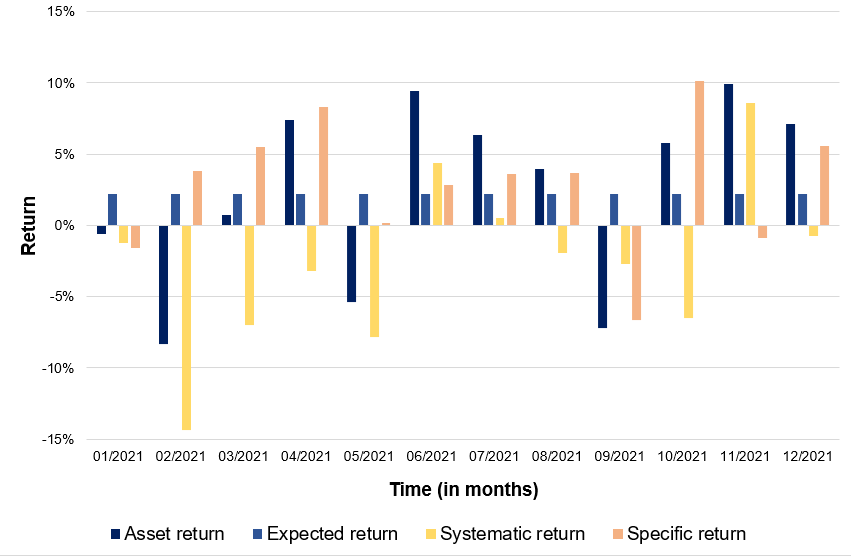
We analyze the decomposition of returns on Apple stocks. Figure 1 gives for every month of 2021 the decomposition of Apple stock returns into three parts: expected return, market factor (systematic return) and an idiosyncratic component (specific return). We used historical price downloaded from the Bloomberg terminal for the period 1999-2022.

Figure 1. Decomposition of Apple stock returns:
expected return, systematic return and specific return.
Decomposition of asset returns Computation by the author (data: Bloomberg).

You can download below the Excel file which illustrates the decomposition of returns on Apple stocks.

Why should I be interested in this post?

Investors will be less influenced by single incidents if they possess a range of firm stocks across several industries, as well as other types of assets in a number of asset classes, such as bonds and stocks.

An investor who only bought telecommunication equities, for example, would be exposed to a high amount of unsystematic risk (also known as idiosyncratic risk). A concentrated portfolio can have an impact on its performance. This investor would spread out telecommunication-specific risks by adding uncorrelated positions to their portfolio, such as firms outside of the telecommunication market.

Useful resources

Academic research

Evans, J.L., Archer, S.H. 1968. Diversification and the Reduction of Dispersion: An Empirical Analysis. The Journal of Finance, 23(5): 761–767.

Markowitz, H. 1952. Portfolio Selection. The Journal of Finance, 7(1): 77-91.

Mossin, J. 1966. Equilibrium in a Capital Asset Market. Econometrica, 34(4): 768-783.

Sharpe, W.F. 1963. A Simplified Model for Portfolio Analysis. Management Science, 9(2): 277-293.

Sharpe, W.F. 1964. Capital Asset Prices: A Theory of Market Equilibrium under Conditions of Risk. The Journal of Finance, 19(3): 425-442.

Tole T.M. 1982. You can’t diversify without diversifying. The Journal of Portfolio Management. Jan 1982, 8 (2) 5-11.

About the author

The article was written in April 2022 by Youssef LOURAOUI (Bayes Business School, MSc. Energy, Trade & Finance, 2021-2022).

Systematic risk

April 1, 2022 by Youssef LOURAOUI

In this article, Youssef LOURAOUI (Bayes Business School, MSc. Energy, Trade & Finance, 2021-2022) presents the systematic risk of financial assets, a key concept in asset pricing models and investment management theories more generally.

This article is structured as follows: we introduce the concept of systematic risk. We then explain the mathematical foundation of this concept. We present an economic understanding of market risk on recent events.

Portfolio Theory and Risk

Markowitz (1952) and Sharpe (1964) developed a framework on risk based on their significant work in portfolio theory and capital market theory. All rational profit-maximizing investors seek to possess a diversified portfolio of risky assets, and they borrow or lend to get to a risk level that is compatible with their risk preferences under a set of assumptions. They demonstrated that the key risk measure for an individual asset is its covariance with the market portfolio under these circumstances (the beta).

The fraction of an individual asset’s total variance attributable to the variability of the total market portfolio is referred to as systematic risk, which is assessed by the asset’s covariance with the market portfolio. Systematic risk can be decomposed into the following categories:

Interest rate risk

We are aware that central banks, such as the Federal Reserve, periodically adjust their policy rates in order to boost or decrease the rate of money in circulation in the economy. This has an effect on the interest rates in the economy. When the central bank reduces interest rates, the money supply expands, allowing companies to borrow more and expand, and when the policy rate is raised, the reverse occurs. Because this is cyclical in nature, it cannot be diversified.

Inflation risk

When inflation surpasses a predetermined level, the purchasing power of a particular quantity of money reduces. As a result of the fall in spending and consumption, overall market returns are reduced, resulting in a decline in investment.

Exchange Rate Risk

As the value of a currency reduces in comparison to other currencies, the value of the currency’s returns reduces as well. In such circumstances, all companies that conduct transactions in that currency lose money, and as a result, investors lose money as well.

Geopolitical Risks

When a country has significant geopolitical issues, the country’s companies are impacted. This can be mitigated by investing in multiple countries; but, if a country prohibits foreign investment and the domestic economy is threatened, the entire market of investable securities suffers losses.

Natural disasters

All companies in countries such as Japan that are prone to earthquakes and volcanic eruptions are at risk of such catastrophic calamities.

Following the Capital Asset Pricing Model (CAPM), the return on asset i, denoted by R_i can be decomposed as

img_SimTrade_return_decomposition

Where:

R_i the return of asset i
E(R_i) the risk premium of asset i
β_i the measure of the risk of asset i
R_M the return of the market
E(R_M) the risk premium of the market
R_M – E(R_M) the market factor
ε_i represent the specific part of the return of asset i

The beta of the asset with the market is computed as:

Beta

Where:

σ_i,m : the covariance of the asset return with the market return
σ_m² : the variance of market return

The total risk of the asset measured by the variance of asset returns can be computed as:

Decomposition of total risk

Where:

β_i² * σ_m² = systematic risk
σ_εi² = specific risk

In this decomposition of the total variance, the first component corresponds to the systematic risk and the second component to the specific risk.

Systematic risk analysis in recent times

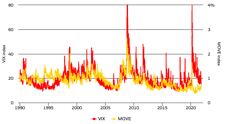
The volatility chart depicts the evolution of implied volatility for the S&P 500 and US Treasury bonds – the VIX and MOVE indexes, respectively. Implied volatility is the price of future volatility in the option market. Historically, the two markets have been correlated during times of systemic risk, like as in 2008 (Figure 1).

Figure 1. Volatility trough time (VIX and MOVE index).

Sources: BlackRock Risk and Quantitative Analysis and BlackRock Investment Institute, with data from Bloomberg and Bank of America Merrill Lynch, October 2021 (BlackRock, 2021).

The VIX index has declined following a spike in September amid the equity market sell-off. It has begun to gradually revert to pre-Covid levels. The periodic, albeit brief, surges throughout the year underscore the underlying fear about what lies beyond the economic recovery and the possibility of a wide variety of outcomes. The MOVE index — a gauge of bond market volatility – has remained relatively stable in recent weeks, despite the rise in US Treasury yields to combat the important monetary policy to combat the effect of the pandemic. This could be a reflection of how central banks’ purchases of government bonds are assisting in containing interest rate volatility and so supporting risk assets (BlackRock, 2021).

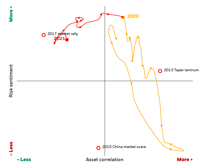
The regime map depicts the market risk environment in two dimensions by plotting market risk sentiment and the strength of asset correlations (Figure 2).

Figure 2. Regime map for market risk environment.

Source: BlackRock Risk and Quantitative Analysis and BlackRock Investment Institute, October 2021 (BlackRock, 2021).

Positive risk sentiment means that riskier assets, such as equities, are outperforming less risky ones. Negative risk sentiment means that higher-risk assets underperform lower-risk assets.

Due to the risk of fast changes in short-term asset correlations, investors may find it challenging to guarantee their portfolios are correctly positioned for the near future. When asset correlation is higher (as indicated by the right side of the regime map), diversification becomes more difficult and risk increases. When asset prices are less correlated (on the left side of the map), investors have greater diversification choices.

When both series – risk sentiment and asset correlation – are steady on the map, projecting risk and return becomes easier. However, when market conditions are unpredictable, forecasting risk and return becomes substantially more difficult. The map indicates that we are still in a low-correlation environment with a high-risk sentiment, which means that investors are rewarded for taking a risk (BlackRock, 2021). In essence, investors should use diversification to reduce the specific risk of their holding coupled with macroeconomic fundamental analysis to capture the global dynamics of the market and better understand the sources of risk.

Why should I be interested in this post?

Market risks fluctuate throughout time, sometimes gradually, but also in some circumstances dramatically. These adjustments typically have a significant impact on the right positioning of a variety of different types of investment portfolios. Investors must walk a fine line between taking enough risks to achieve their objectives and having the proper instruments in place to manage sharp reversals in risk sentiment.

Useful resources

Academic research

Markowitz, H. 1952. Portfolio Selection. The Journal of Finance, 7(1): 77-91.

Mossin, J. 1966. Equilibrium in a Capital Asset Market. Econometrica, 34(4): 768-783.

Sharpe, W.F. 1963. A Simplified Model for Portfolio Analysis. Management Science, 9(2): 277-293.

Sharpe, W.F. 1964. Capital Asset Prices: A Theory of Market Equilibrium under Conditions of Risk. The Journal of Finance, 19(3): 425-442.

Business analysis

BlackRock, 2021. Market risk monitor

About the author

The article was written in April 2022 by Youssef LOURAOUI (Bayes Business School, MSc. Energy, Trade & Finance, 2021-2022).

Implementing Black-Litterman asset allocation model

March 21, 2022 by Youssef LOURAOUI

In this article, Youssef Louraoui (Bayes Business School, MSc. Energy, Trade & Finance, 2021-2022) presents an implementation of the Black-Litterman model, used to determine the expected return of a portfolio by integrating investor’s views regarding the performance of the underlying assets selected in the investment portfolio.

This article follows the following structure: first, we introduce the Black-Litterman model. We then present the mathematical foundations of this model. We conclude with an explanation of the methodology to build the spreadsheet with the results obtained. You will find in this post an Excel spreadsheet which implement the model.

Introduction

The Black-Litterman asset allocation model, established for the first time in the early 1990’s by Fischer Black and Robert Litterman, is a sophisticated strategy for dealing with unintuitive, highly concentrated, and input-sensitive portfolios. The most likely reason that more portfolio managers do not use the Markowitz model, which maximises return for a given degree of risk, is input sensitivity, a well-documented issue with mean-variance optimization.

The Black-Litterman Model employs a Bayesian technique to integrate an investor’s subjective views of expected returns on one or more assets with the market equilibrium vector (prior distribution) of expected returns to obtain a new, mixed estimate of expected returns. The new vector of returns (the posterior distribution) is a weighted complex average of the investor’s views and market equilibrium.

Mathematical foundation

The idea of the Black Litterman estimates is not to find the optimum portfolio weights as in the Markowitz optimization framework, but instead to find the expected return that would be used as an input to compute the optimum portfolio weights. This approach is referred as reversion portfolio optimization technique. The idea behind is that optimum weights are already observed in the market and captured in the market portfolio. We can approach the reasoning by maximizing the following utility function adjusted to the risk:

img_SimTrade_mathematical_foundation_Black_Litterman_6

w^T = transposed of portfolio weights
Π = Implied equilibrium excess return vector
A = price of risk or risk aversion factor
Σ = variance-covariance matrix

We take the partial derivative of U in terms of weights (w) and we derive the following expression:

img_SimTrade_mathematical_foundation_Black_Litterman_5

By setting the partial derivative equal to zero, we can maximize the utility function in term of weights. The proposed approach in the Black Litterman approach is that instead of seeking the optimal weights, which are incorporated in the market portfolio and thus computable via the market capitalization of the equities in the portfolio, we’ll isolate the Π (implied equilibrium excess return) to obtain the optimal expected returns for the portfolio:

We can deconstruct the Black-Litterman model as

img_SimTrade_mathematical_foundation_Black_Litterman_3

τ= scalar
P = Linking matrix
∑ = Variance-covariance matrix
Π= implied equilibrium excess return
A = Price of risk
w = weight vector
Ω = uncertainty of views

The first term of the formula is introduced in order to respect the constraint that the portfolio weights should be equal to one:

The second term of the formula is to compute a weighted average of the implied equilibrium excess return adjusted to the uncertainty of the returns by the view vector weighted with the uncertainty of views:

The final output E(R) is a vector of return n x 1 that represent the equilibrium returns of the market adjusted to investors views.

Implementation of the Black-Litterman asset allocation model in practice

To model a Black-Litterman portfolio allocation, we obtained a large time series to obtain useful results by downloading the equivalent of 23 years of market data from a data provider (in this example, Bloomberg). We generate the variance-covariance matrix after obtaining all necessary statistical data, which includes the expected return and volatility indicated by the standard deviation of the returns for each stock during the provided period.

The data is derived from the Bloomberg terminal. The first step is to calculate the logarithmic returns and excess returns on the selected assets (returns minus the risk-free rate). After calculating the logarithmic returns on each asset, we can estimate the capital asset pricing model’s returns (CAPM) expected returns. This information will be used to calculate the Black-Litterman expected returns on a comparative basis.

1. The first input for the model is the price of risk A, which represents the risk aversion of investor and is obtained by subtracting the expected return of the market the risk-free rate and divided by the variance of the market:

img_SimTrade_Black_Litterman_formulas_for_spreadsheet_1

E(r_m)= expected market returns
r_f = risk-free rate
σ²_m = variance of market

2. We extract the respective market capitalization of each security to obtain their market weights in the portfolio. Given that our investable universe is made of five stocks, we can retrieve their respective market capitalization and compute the weights of each stock in relation to the sum of total market-capitalization in the portfolio.

img_SimTrade_Black_Litterman_formulas_for_spreadsheet_2

Table 1 depicts the optimal weights obtained from their respective market capitalisation, coupled with the respective expected return and volatility.

Table 1. Asset characteristics of Apple, Amazon, Microsoft, Goldman Sachs, and Pfizer.

img_SimTrade_Black_Litterman_spreadsheet_2

Source: computation by the author.

3. We compute the variance-covariance matrix of logarithmic returns using the data analysis tool pack available in Excel (Table 2).

Table 2. Variance-covariance matrix of asset returns

img_SimTrade_Black_Litterman_spreadsheet_5

Source: computation by the author.

4. We compute the implied equilibrium excess return (Π) as the matrix calculation of the price of risk (A) times the matrix multiplication of the weights computed in step 4 times the variance-covariance matrix computed in step 3.

img_SimTrade_Black_Litterman_formulas_for_spreadsheet_3

Π= implied equilibrium excess return
A = Price of risk
w = weight vector

5. The views are incorporated into the model. To achieve this, we provide three views to include into the model. If there are no views, the values will correspond to the market portfolio. The investment manager’s views for the expected return on certain of the portfolio’s assets regularly diverge from the Implied Equilibrium Return Vector (), which serves as the market-neutral starting point for the Black-Litterman model that quantifies the uncertainty associated with each view. The Black-Litterman Model can be used to depict such views in absolute or relative terms. As an illustration, let us suppose that the real and simulated portfolio will have the same views:

View 1: Apple will outperform Microsoft by .05 percent
View 2: Amazon will outperform Microsoft by .1 percent
View 3: Apple will outperform Amazon by .05 percent

To incorporate the vector Q of views, we create a link matrix P where the rows sum to zero. Figure 3 depicts the workings done in the spreadsheet.

Table 3. Views vector and Link Matrix (P)

img_SimTrade_Black_Litterman_spreadsheet_1

Source: computation by the author.

6. We compute omega to determine the degree of uncertainty associated with the views. While Black-Litterman paper used a value of tau equal to 0.25, an important number of academics went for calculating the tau equal to one. For the sake of simplifying the model, consider tau to be equal to one. This input is obtained by multiplying the Linking matrix by the variance-covariance matrix and transposing the Linking matrix (P).

img_SimTrade_Black_Litterman_formulas_for_spreadsheet_4

τ= scalar
P = Linking matrix
∑ = Variance-covariance matrix

7. We integrate all the values computed previously in the Black-Litterman model. Table 4 depicts the results obtained via the Black-Litterman allocation model.

Table 4. Results of the Black-Litterman allocation

img_SimTrade_Black_Litterman_spreadsheet_4

Source: computation by the author.

We can see that the results converge slightly to those from CAPM. Additionally, we can see that the views are reflected in the Black-Litterman expected returns. As a result, we can determine whether or not each view is satisfied. Indeed, Apple outperforms Amazon and Microsoft, while Amazon outperforms Microsoft.

You can download an Excel file to help you construct a portfolio via the Black-Litterman allocation model.

Why should I be interested in this post?

Modern Portfolio Theory is at the heart of modern finance, shaping the modern investing landscape. MPT has become the cornerstone of current financial theory and practice. MPT’s thesis is that winning the market is difficult and requires diversification and taking higher-than-average risks.

MPT has been around for nearly sixty years and shows no signs of slowing down. His theoretical contributions paved the way for more portfolio theory study. But Markowitz’s portfolio theory is sensitive to and depends on further ‘probabilistic’ expansion. This paper expanded on Markowitz’s previous work by incorporating investor views into the asset allocation process.

Useful resources

Academic research

Black, F. and Litterman, R. 1990. Asset Allocation: Combining Investors Views with Market Equilibrium. Goldman Sachs Fixed Income Research working paper

Black, F. and Litterman, R. 1991. Global Asset Allocation with Equities, Bonds, and Currencies. Goldman Sachs Fixed Income Research working paper

Black, F. and Litterman, R. 1992. Global Portfolio Optimization.Financial Analysts Journal, 28-43.

Idzorek, T.M. 2002. A step-by-step guide to Black-Litterman model. Incorporating user-specified confidence levels. Working Paper, 2-11.

Markowitz, H., 1952. Portfolio Selection. The Journal of Finance, 7(1): 77-91.

About the author

The article was written in Mars 2022 by Youssef LOURAOUI (Bayes Business School, MSc. Energy, Trade & Finance, 2021-2022).

Implementing Markowitz asset allocation model

March 20, 2022 by Youssef LOURAOUI

In this article, Youssef LOURAOUI (Bayes Business School, MSc. Energy, Trade & Finance, 2021-2022) explains how to implement the Markowitz asset allocation model. This model is used to determine optimal asset portfolios based on the risk-return trade-off.

This article follows the following structure: first, we introduce the Markowitz model. We then present the mathematical foundations of this model. We conclude with an explanation of the methodology to build the spreadsheet with the results obtained. You will find in this post an Excel spreadsheet which implements the Markowitz asset allocation model.

Introduction

Markowitz’s work is widely regarded as a pioneer work in financial economics and corporate finance due to its theoretical foundations and applicability in the financial sector. Harry Markowitz received the Nobel Prize in 1990 for his contributions to these disciplines, which he outlined in his 1952 article “Portfolio Selection” published in The Journal of Finance. His major work established the foundation for what is now commonly referred to as “Modern Portfolio Theory” (MPT).

To find the portfolio’s minimal variance, the Markowitz model uses a constrained optimization strategy. The goal of the Markowitz model is to take into account the expected return and volatility of the assets in the investable universe to provide an optimal weight vector that indicates the best allocation for a given level of expected return or the best allocation for a given level of volatility. The expected return, volatility (standard deviation of expected return), and the variance-covariance matrix to reflect the co-movement of each asset in the overall portfolio design are the major inputs for this portfolio allocation model for an n-asset portfolio. We’ll go over how to use this complex method to find the best portfolio weights in the next sections.

Mathematical foundations

With the following notations:

w_P = vector of asset weights of the portfolio
μ_P = desired level of expected return
e = identity vector
μ = vector of expected returns
V = variance-covariance matrix of returns
V^-1 = inverse of the variance-covariance matrix
t = transpose operation for vectors and matrices

A, B and C are intermediate parameters computed below:

img_SimTrade_implementing_Markowitz_2

The variance of the optimal portfolio is computed as follows

img_SimTrade_implementing_Markowitz_3

To calculate the standard deviation of the optimal portfolio, we take the square root of the variance.

Implementation of the Markowitz asset allocation model in practice

Table 1. Asset characteristics of Apple, Amazon, Microsoft, Goldman Sachs, and Pfizer.
img_SimTrade_implementing_Markowitz_spreadsheet_1
Source: computation by the author.

We use the data analysis tool pack supplied in Excel to run a variance-covariance matrix for ease of computation (Table 2).

Table 2. Variance-covariance matrix of asset returns.
img_SimTrade_implementing_Markowitz_spreadsheet_4
Source: computation by the author.

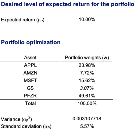
We can start the optimization task by setting a desirable expected return after computing the expected return, volatility, and the variance-covariance matrix of expected return. With the data that is fed into the appropriate cells, the model will complete the optimization task. For a 10% desired expected return, we get the following results (Table 3).

Table 3. Asset weights for an optimal portfolio.
img_SimTrade_implementing_Markowitz_spreadsheet_2
Source: computation by the author.

Figure 1. Markowitz efficient portfolio frontier.
img_SimTrade_implementing_Markowitz_spreadsheet_3
Source: computation by the author.

You can download the Excel file below to use the Markowitz portfolio allocation model.

Why should I be interested in this post?

Modern Portfolio Theory (MPT) is at the heart of modern finance, shaping the modern investing landscape. MPT has become the cornerstone of current financial theory and practice. MPT has been around for nearly sixty years and shows no signs of slowing down. His theoretical contributions paved the way for more portfolio theories. This post helps you to grasp the theoretical model and its implementation.

Useful resources

Academic research

Petters, A. O., and Dong, X. 2016. An Introduction to Mathematical Finance and Applications. Springer Undergraduate Texts in Mathematics and Technology.

Markowitz, H., 1952. Portfolio Selection. The Journal of Finance, 7(1): 77-91.

About the author

The article was written in Mars 2022 by Youssef LOURAOUI (Bayes Business School, MSc. Energy, Trade & Finance, 2021-2022).

Systematic risk and specific risk

November 30, 2021 by Youssef LOURAOUI

In this article, Youssef LOURAOUI (Bayes Business School, MSc. Energy, Trade & Finance, 2021-2022) presents the systematic risk and specific risk of financial assets, two fundamental concepts in asset pricing models and investment management theories more generally.

This article is structured as follows: we introduce the concept of systematic and specific risk. We then explain the mathematical foundation of this concept. We finish with an insight that sheds light on the relationship between diversification and risk reduction.

Portfolio Theory and Risk

The fraction of an individual asset’s total variance attributable to the variability of the total market portfolio is referred to as systematic risk, which is assessed by the asset’s covariance with the market portfolio. In the article systematic risk, we develop the economic sources of systematic risk: interest rate risk, inflation risk, exchange rate risk, geopolitical risk, and natural risk.

Additionally, due to the asset’s unique characteristics, an individual asset exhibits variance that is unrelated to the market portfolio (the asset’s non-market variance). Specific risk is the term for non-market variance, and it is often seen as minor because it can be eliminated in a large diversified portfolio. In the article specific risk, we develop the economic sources of specific risk: business risk and financial risk.

Mathematical foundations

Following the Capital Asset Pricing Model (CAPM), the return on asset i, denoted by R_i can be decomposed as

img_SimTrade_return_decomposition

Where:

R_i the return of asset i
E(R_i) the expected return of asset i
β_i the measure of the risk of asset i
R_M the return of the market
E(R_M) the expected return of the market
R_M – E(R_M) the market factor
ε_i the specific part of the return of asset i

The beta of the asset with the market is computed as:

Beta

Where:

σ_i,m : the covariance of the asset return with the market return
σ_m² : the variance of market return

Total risk can be deconstructed into two main blocks:

Total risk formula

The total risk of the asset measured by the variance of asset returns can be computed as:

Decomposition of total risk

Where:

β_i² * σ_m² = systematic risk
σ_εi² = specific risk

In this decomposition of the total variance, the first component corresponds to the systematic risk and the second component to the specific risk.

Effect of diversification on portfolio risk

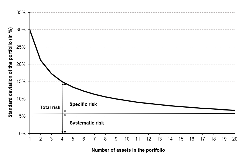
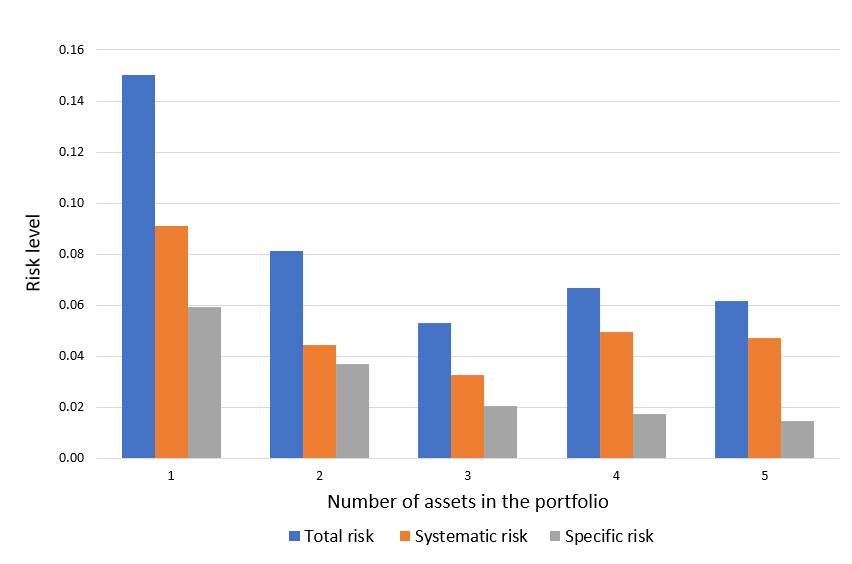
Diversification’s objective is to reduce the portfolio’s standard deviation. This assumes an imperfect correlation between securities. Ideally, as investors add securities, the portfolio’s average covariance decreases. How many securities must be included to create a portfolio that is completely diversified? To determine the answer, investors must observe what happens as the portfolio’s sample size increases by adding securities with some positive correlation. Figure 1 illustrates the effect of diversification on portfolio risk, more precisely on total risk and its two components (systematic risk and specific risk).

Figure 1. Effect of diversification on portfolio risk

Source: Computations from the author.

The critical point is that by adding stocks that are not perfectly correlated with those already held, investors can reduce the portfolio’s overall standard deviation, which will eventually equal that of the market portfolio. At that point, investors eliminated all specific risk but retained market or systematic risk. There is no way to completely eliminate the volatility and uncertainty associated with macroeconomic factors that affect all risky assets. Additionally, investors can reduce systematic risk by diversifying globally rather than just within the United States, as some systematic risk factors in the United States market (for example, US monetary policy) are not perfectly correlated with systematic risk variables in other countries such as Germany and Japan. As a result, global diversification eventually reduces risk to a global systematic risk level.

You can download below two Excel files which illustrate the effect of diversification on portfolio risk.

The first Excel file deals with the case of independent assets with the same profile (risk and expected return).

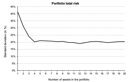
Figure 2 depicts the risk reduction of total risk in as we increase the number of assets in the portfolio. We manage to reduce half of the overall portfolio volatility by adding five assets to the portfolio. However, the decrease becomes more and more marginal as we add more assets.

Figure 2. Risk reduction of the portfolio. img_SimTrade_systematic_specific_risk_1 Source: Computations from the author.

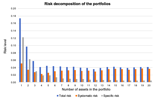
Figure 3 depicts the overall risk reduction of a portfolio. The benefit of diversification are more evident when we add the first 5 assets in the portfolio. As depicted in Figure 2, the diversification starts to fade at a certain point as we keep adding more assets in the portfolio. It can be seen in this figure how the specific risk is considerably reduced as we add more assets because of the effect of diversification. Systematic risk (market risk) is more constant and doesn’t change drastically as we diversify the portfolio. Overall, we can clearly see that diversification helps decrease the total risk of a portfolio considerably.

Figure 3. Risk decomposition of the portfolio. img_SimTrade_systematic_specific_risk_2 Source: Computations from the author.

The second Excel file deals with the case of dependent assets with the different characteristics (expected return, volatility, and market beta).

Academic research

A series of studies examined the average standard deviation for a variety of portfolios of randomly chosen stocks with varying sample sizes. Evans and Archer (1968) and Tole (1982) calculated the standard deviation for portfolios up to a maximum of twenty stocks. The results indicated that the majority of the benefits of diversification were obtained relatively quickly, with approximately 90% of the maximum benefit of diversification being obtained from portfolios of 12 to 18 stocks. Figure 1 illustrates this effect graphically.

This finding has been modified in two subsequent studies. Statman (1987) examined the trade-off between diversification benefits and the additional transaction costs associated with portfolio expansion. He concluded that a portfolio that is sufficiently diversified should contain at least 30–40 stocks. Campbell, Lettau, Malkiel, and Xu (2001) demonstrated that as the idiosyncratic component of an individual stock’s total risk (specific risk) has increased in recent years, it now requires a portfolio to contain more stocks to achieve the same level of diversification. For example, they demonstrated that the level of diversification possible in the 1960s with only 20 stocks would require approximately 50 stocks by the late 1990s (Reilly and Brown, 2012).

Figure 4. Effect of diversification on portfolio risk Source: Computation from the author.

You can download below the Excel file which illustrates the effect of diversification on portfolio risk with real assets (Apple, Microsoft, Amazon, etc.). The effect of diversification on the total risk of the portfolio is already significant with the addition of few stocks.

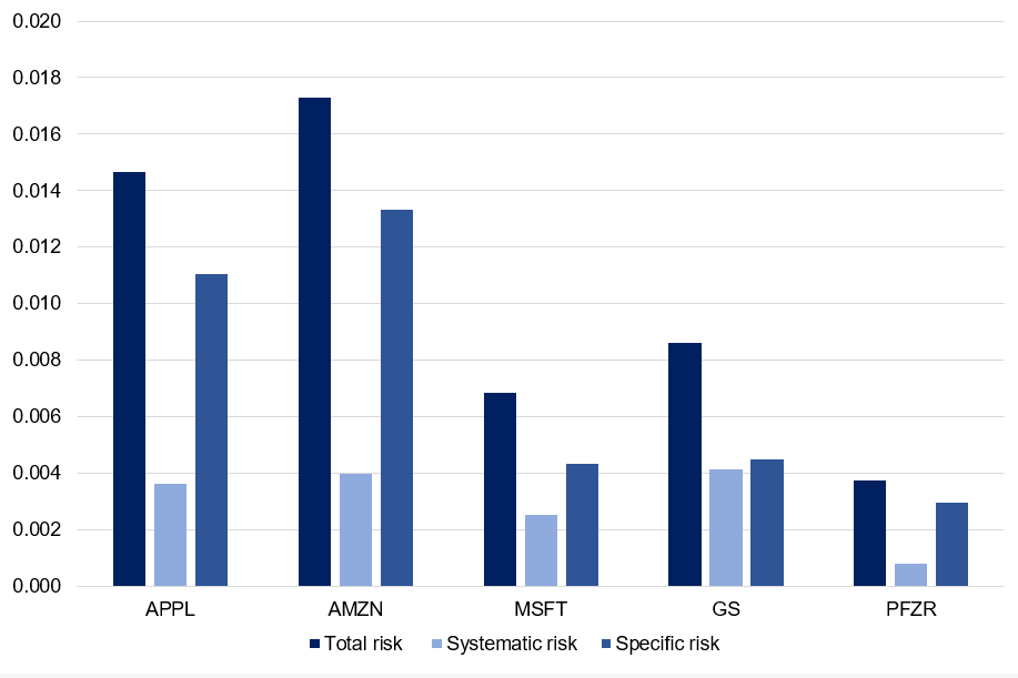
We can appreciate the decomposition of total risk in the below figure with real asset. We can appreciate how asset with low beta had the lowest systematic out of the sample analyzed (i.e. Pfizer). For the whole sample, specific risk is a major concern which makes the major component of risk of each stock. This can be mitigated by holding a well-diversified portfolio that can mitigate this component of risk. Figure 5 depicts the decomposition of total risk for assets (Apple, Microsoft, Amazon, Goldman Sachs and Pfizer).

Figure 5. Decomposition of total risk Source: Computation from the author.

You can download below the Excel file which deconstructs the risk of assets (Apple, Microsoft, Amazon, Goldman Sachs, and Pfizer).

Why should I be interested in this post?

If you’re an investor, understanding the source of risk is essential in order to build balanced portfolios that can withstand market corrections and downturns.

If you are a business school or university undergraduate or graduate student, this content will help you in broadening your knowledge of finance.

Useful resources

Academic research

Campbell, J.Y., Lettau, M., Malkiel, B.G. and Xu, Y. 2001. Have Individual Stocks Become More Volatile? An Empirical Exploration of Idiosyncratic Risk. The Journal of Finance, 56: 1-43.

Evans, J.L., Archer, S.H. 1968. Diversification and the Reduction of Dispersion: An Empirical Analysis. The Journal of Finance, 23(5): 761–767.

Markowitz, H. 1952. Portfolio Selection. The Journal of Finance, 7(1): 77-91.

Mossin, J. 1966. Equilibrium in a Capital Asset Market. Econometrica, 34(4): 768-783.

Reilly, R.K., Brown C.K. 2012. Investment Analysis & Portfolio Management, Tenth Edition. 239-245.

Sharpe, W.F. 1963. A Simplified Model for Portfolio Analysis. Management Science, 9(2): 277-293.

Sharpe, W.F. 1964. Capital Asset Prices: A Theory of Market Equilibrium under Conditions of Risk. The Journal of Finance, 19(3): 425-442.

Statman, M. 1987. How Many Stocks Make a Diversified Portfolio?. The Journal of Financial and Quantitative Analysis, 22(3), 353–363.

Tole T.M. 1982. You can’t diversify without diversifying. The Journal of Portfolio Management. Jan 1982, 8 (2) 5-11.

About the author

The article was written in November 2021 by Youssef LOURAOUI (Bayes Business School, MSc. Energy, Trade & Finance, 2021-2022).

Portfolio

November 26, 2021 by Youssef LOURAOUI

In this article, Youssef LOURAOUI (Bayes Business School, MSc. Energy, Trade & Finance, 2021-2022) elaborates on the concept of portfolio, which is a basic element in asset management.

This article is structured as follows: we introduce the concept of portfolio. We give the basic modelling to define and characterize a portfolio. We then expose the different types of portfolios that investors can rely on to meet their financial goals.

Introduction

An investment portfolio is a collection of assets that an investor owns. These assets can be individual assets such as bonds and stocks or baskets of assets such as mutual funds or exchange-traded funds (ETFs). In a nutshell, this refers to any asset that has the potential to increase in value or generate income. When building a portfolio, investors usually consider the expected return and risk. A well-balanced portfolio includes a variety of investments.

Modelling of portfolios

Portfolio weights

At a point of time, a portfolio is fully defined by the weights (w) of the assets of the universe considered (N assets).

Portfolio weights

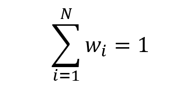
The sum of the portfolio weights adds up to one (or 100%):

Sum of the portfolio weights

The weight of a given asset i can be positive (for a long position in the asset), equal to zero (for a neutral position in the asset) or negative (for a short position in the asset):

Asset weight for a long position

Asset weight for a neutral position

Asset weight for a short position

Short selling is the process of selling a security without owning it. By definition, a short sell occurs when an investor borrows a stock, sells it, and then buys it later back to repay the lender.

The equally-weighted portfolio is defined as the portfolio with weights that are evenly distributed across the number of assets held:

Equally-weigthed portfolio

Portfolio return: the case of two assets

Over a given period of time, the returns on assets 1 and 2 are equal to r₁ and r₂. In the two-asset portfolio case, the portfolio return r_P is computed as

Return of a 2-asset portfolio

The expected return of the portfolio E(r_P) is computed as

Expected return of a 2-asset portfolio

The standard deviation of the portfolio return, σ(r_P) is computed as

Standard deviation of a 2-asset portfolio return

where:

σ₁ = standard deviation of asset 1
σ₂ = standard deviation of asset 2
σ_1,2 = covariance of assets 1 and 2
ρ_1,2 = correlation of assets 1 and 2

Investing in asset classes with low or no correlation to one another can help you increase portfolio diversification and reduce portfolio volatility. While diversification cannot guarantee a profit or eliminate the risk of investment loss, the ideal scenario is to have a mix of uncorrelated asset classes in order to reduce overall portfolio volatility and generate more consistent long-term returns. Correlation is depicted mathematically as the division of the covariance between the two assets by the individual standard deviation of the asset. Correlation is a more interpretable metric than covariance because it’s measurable within a defined rank. Correlation is measured between -1 and 1, with a high positive correlation showing that the assets move in tandem, while negative correlation depicts securities that have contrary price movements. The holy grail of investing is to invest in securities that offer a low correlation of the portfolio as a whole.

where:

σ_1,2 = covariance of assets 1 and 2
σ₁ = standard deviation of asset 1
σ₂ = standard deviation of asset 2

Correlation is a more interpretable metric than covariance because it’s measurable within a defined rank. Correlation is measured between -1 and 1, with high positive correlation showing that the assets move in tandem, while negative correlation depicts securities that have contrary price movements. The holy grail of investing is to invest in securities that offer a low correlation of the portfolio as a whole.

You can download an Excel file to help you construct a portfolio and compute the expected return and variance of a two-asset portfolio. Just introduce the inputs in the model and the calculations will be performed automatically. You can even draw the efficient frontier to plot the different combinations of portfolios that optimize the risk-return trade-off (to minimize the risk for a given level of expected return or to maximize the expected return for a given level of risk).

Portfolio return: the case of N assets

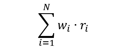
Over a given period of time, the return on asset i is equal to r_i. The portfolio return can be computed as

Portfolio return

The expression of the portfolio return is then used to compute two important portfolio characteristics for investors: the expected performance measured by the average return and the risk measured by the standard deviation of returns.

The expected return of the portfolio is given by

Expected portfolio return

Because relying on multiple assets can get extremely computationally heavy, we can refer to the matrix form for more straightforward use. We basically compute the vector of weight with the vector of returns (NB: we have to pay attention to the dimension and to the properties of matrix algebra).

w = weight vector
r = returns vector

The standard deviation of returns of the portfolio is given by the following equivalent formulas:

Standard deviation of portfolio return

w_i = weight of asset i
w_j = weight of asset j
σ_i = standard deviation of asset i
σ_j = standard deviation of asset j
ρ_i,j = correlation of asset i,j

Standard deviation of portfolio return

where:

w_i² = squared weight of asset I
σ_i² = variance of asset i
w_i = weight of asset i
w_j = weight of asset j
σ_i = standard deviation of asset i
σ_j = standard deviation of asset j
ρ_i,j = correlation of asset i,j

We can use the matrix form for a more straightforward application due to the computational burden associated with relying on multiple assets. Essentially, we multiply the vector of weights with the variance-covariance matrix and the transposed weight vector (NB: we must pay attention to the dimension and to the properties of matrix algebra).

w = weight vector
∑ = variance-covariance matrix
w’ = transpose of weight vector

You can get an Excel file that will help you build a portfolio and calculate the expected return and variance of a three-asset portfolio. Simply enter the data into the model, and the calculations will be carried out automatically. You can even use the efficient frontier to plot the various portfolio combinations that best balance risk and reward (to minimize the risk for a given level of expected return or to maximize the expected return for a given level of risk).

Basic principles on portfolio construction

Diversify

Diversification, a core principle of Markowitz’s portfolio selection theory, is a risk-reduction strategy that entails allocating assets among a variety of financial instruments, sectors, and other asset classes (Markowitz, 1952). In more straightforward terms, it refers to the concept “don’t put all your eggs in one basket.” If the basket is dropped, all eggs are shattered; if many baskets are used, the likelihood of all eggs being destroyed is significantly decreased. Diversification may be accomplished by investments in a variety of companies, asset types (e.g., bonds, real estate, etc.), and/or commodities such as gold or oil.

Diversification seeks to enhance returns while minimizing risk by investing in a variety of assets that will react differently to the same event(s). Portfolio diversification methods should include not just diverse stocks inside and outside of the same industry, but also diverse asset classes, such as bonds and commodities. When there is an imperfect connection between assets (lower than one), the diversification effect occurs. It is a critical and successful risk mitigation method since risk mitigation may be accomplished without jeopardizing profits. As a result, any prudent investor who is cautious (or ‘risk averse’) will diversify to a certain extent.

Portfolio Asset Allocation

The term “asset allocation” refers to the proportion of stocks, bonds, and cash in a portfolio. Depending on your investing strategy, you’ll determine the percentage of each asset type in your portfolio to achieve your objectives. As markets fluctuate over time, your asset allocation is likely to go out of balance. For instance, if Tesla’s stock price increases, the percentage of your portfolio allocated to stocks will almost certainly increase as well.

Portfolio Rebalancing

Rebalancing is a term that refers to the act of purchasing and selling assets in order to restore your portfolio’s asset allocation to its original state and avoid disrupting your plan.

Reduce investment costs as much as possible

Commission fees and management costs are significant expenses for investors. This is especially important if you frequently purchase and sell stocks. Consider using a discount brokerage business to make your investment. Clients are charged much lesser fees by these firms. Also, when investing for the long run, it is advisable to avoid making judgments based on short-term market fluctuations. To put it another way, don’t sell your stocks just because they’ve taken a minor downturn in the near term.

Invest on a regular basis

It is critical to invest on a regular basis in order to strengthen your portfolio. This will not only build wealth over time, but it will also develop the habit of investing discipline.

Buying in the future

It’s possible that you have no idea how a new stock will perform when you buy it. To be on the safe side, avoid putting your entire position to a single investment. Start with a little investment in the stock. If the stock’s performance fulfils your expectations, you can gradually increase your investments until you’ve covered your entire position.

Types of portfolio

We detail below the different types of portfolios usually proposed by financial institutions that investors can rely on to meet their financial goals.

Aggressive Portfolio

As the name implies, an aggressive portfolio is one of the most frequent types of portfolio that takes a higher risk in the pursuit of higher returns. Stocks in an aggressive portfolio have a high beta, which means they present more price fluctuations compared to the market. It is critical to manage risk carefully in this type of portfolio. Keeping losses to a minimal and taking profits are crucial to success. It is suitable for a high-risk appetite investor.

Defensive Portfolio

A defensive portfolio is one that consists of stocks with a low beta. The stocks in this portfolio are largely immune to market swings. The goal of this type of portfolio is to reduce the risk of losing the principal. Fixed-income securities typically make up a major component of a defensive portfolio. It is suitable for a low-risk appetite investor.

Income Portfolio

Another typical portfolio type is one that focuses on investments that generate income from dividends (for stocks), interests (for bonds) or rents (for real estate). An income portfolio invests in companies that return a portion of their profits to shareholders, generating positive cash flow. It is critical to remember that the performance of stocks in an income portfolio is influenced by the current economic condition.

Speculative Portfolio

Among all portfolio types, a speculative portfolio has the biggest risk. Speculative investments could be made of different assets that possess inherently higher risks. Stocks from technology and health-care companies that are developing a breakthrough product, junk bonds, distressed investments among others might potentially be included in a speculative portfolio. When establishing a speculative portfolio, investors must exercise caution due to the high risk involved.

Hybrid Portfolio

A hybrid portfolio is one that includes passive investments and offers a lot of flexibility. The cornerstone of a hybrid portfolio is typically made up of blue-chip stocks and high-grade corporate or government bonds. A hybrid portfolio provides diversity across many asset classes while also providing stability by combining stocks and bonds in a predetermined proportion.

Socially Responsible Portfolio

A socially responsible portfolio is based on environmental, social, and governance (ESG) criteria. It allows investors to make money while also doing good for society. Socially responsible or ESG portfolios can be structured for any level of risk or investment aim and can be built for growth or asset preservation. The important thing is that they prefer stocks and bonds that aim to reduce or eliminate environmental impact or promote diversity and equality.

Why should I be interested in this post?

Useful resources

Academic research

Mangram, M.E., 2013. A simplified perspective of the Markowitz Portfolio Theory. Global Journal of Business Research, 7(1): 59-70.

Markowitz, H., 1952. Portfolio Selection. The Journal of Finance, 7(1): 77-91.

Business analysis

Edelweiss, 2021.What is a portfolio?

Forbes, 2021.Investing basics: What is a portfolio?

JP Morgan Asset Management, 2021.Glossary of investment terms: Portfolio

About the author

The article was written in November 2021 by Youssef LOURAOUI (Bayes Business School, MSc. Energy, Trade & Finance, 2021-2022).

Introduction

Key elements of the paper

Conclusion

Why should I be interested in this post?

Related posts on the SimTrade blog

Useful resources

Academic research

About the author

Introduction

Academic Literature

Example

Excel file to build the Minimum Volatility Portfolio

Why should I be interested in this post?

Related posts on the SimTrade blog

Useful resources

Academic research

Business analysis

About the author

Introduction

Mathematical foundations

Optimal portfolio application: the case of two assets

Optimal portfolio application: the general case

Why should I be interested in this post?

Related posts on the SimTrade blog

Useful resources

Academic research

About the author

Portfolio Theory and Risk

Sources of specific risk

Business risk

Financial risk

Mathematical foundations

Decomposition of returns

Why should I be interested in this post?

Related posts on the SimTrade blog

Useful resources

Academic research

About the author

Portfolio Theory and Risk

Interest rate risk

Inflation risk

Exchange Rate Risk

Geopolitical Risks

Natural disasters

Systematic risk analysis in recent times

Why should I be interested in this post?

Related posts on the SimTrade blog

Useful resources

Academic research

Business analysis

About the author

Introduction

Mathematical foundation

Implementation of the Black-Litterman asset allocation model in practice

Why should I be interested in this post?

Related posts on the SimTrade blog

Useful resources

Academic research

About the author

Introduction

Mathematical foundations

Implementation of the Markowitz asset allocation model in practice

Why should I be interested in this post?

Related posts on the SimTrade blog

Useful resources

Academic research

About the author

Portfolio Theory and Risk

Mathematical foundations

Effect of diversification on portfolio risk

Academic research

Why should I be interested in this post?

Related posts on the SimTrade blog

Useful resources

Academic research

About the author

Introduction

Modelling of portfolios

Portfolio weights

Portfolio return: the case of two assets