In this article, Frédéric VALOGNES, lecturer, author and Certified European Financial Analyst (CEFA®), examines whether the dynamics of the implied volatility surface may provide a decision-support framework for systematic cash-secured put strategies.

Abstract

The Black-Scholes-Merton model remains one of the most influential developments in modern financial economics. Whilst its mathematical formulation continues to provide the benchmark for pricing European options, one of its central assumptions — namely that volatility remains constant throughout the life of an option — is persistently contradicted by observed market prices.

Rather than constituting a weakness of the model, these discrepancies reveal valuable information regarding investors’ expectations, market sentiment and the pricing of downside risk. The resulting volatility skews and smiles have therefore become essential components of both academic research and professional option trading.

This paper argues that the implied volatility surface should not be viewed solely as a pricing adjustment. Its geometry and, more importantly, its evolution over time may provide additional information capable of assisting investment decisions. Attention is devoted to cash-secured short put strategies, for which the level of implied volatility alone frequently proves insufficient.

Drawing upon preliminary observations obtained from listed CAC 40 index options across several maturities, the article explores whether the dynamics of the implied volatility surface may constitute a useful decision-support indicator. Rather than proposing a predictive pricing model, the objective is to examine whether changes in the shape, slope and term structure of implied volatility can contribute to a more disciplined framework for identifying favourable market environments in which to initiate systematic cash-secured put strategies.

Introduction

Within option markets, implied volatility occupies a rather singular position. Originally introduced as the unknown parameter required to reconcile observed option prices with the Black-Scholes-Merton valuation model, it has progressively evolved from a purely technical pricing input into one of the most closely monitored indicators in financial markets. Today, implied volatility is commonly interpreted not simply as a pricing parameter, but as a market-based measure of uncertainty, reflecting the aggregate expectations of thousands of market participants.

For investors employing cash-secured short put strategies, that is, selling put options while maintaining sufficient cash reserves to purchase the underlying asset if assignment occurs, implied volatility plays an obvious practical role. Higher implied volatility generally translates into higher option premiums, thereby increasing the potential income associated with selling options. This simple observation has encouraged many practitioners to associate elevated implied volatility with favourable selling opportunities.

Experience, however, suggests that such a conclusion is frequently incomplete. Periods characterised by exceptionally high implied volatility often coincide with episodes of considerable financial stress, during which uncertainty continues to increase and option premiums expand further. Entering short option positions solely because implied volatility appears elevated may therefore expose investors to significant mark-to-market losses before market conditions eventually stabilise.

The question addressed in this article is therefore slightly different.

Rather than asking whether implied volatility is high, it may be more appropriate to ask whether the behaviour of the implied volatility surface itself contains additional information capable of assisting investment decisions.

More specifically, can the dynamics of the implied volatility surface, particularly the evolution of the downside volatility skew, provide useful information regarding changing market conditions? Since deep out-of-the-money put options typically incorporate a substantial premium reflecting institutional demand for portfolio insurance, does a progressive flattening of the skew signal that market stress is easing while option premiums remain comparatively attractive?

If such behaviour can be observed consistently, the volatility surface ceases to be merely an output of an option pricing model. Instead, it becomes a potential decision-support framework, capable of complementing more traditional criteria such as premium level, strike selection or time to maturity.

The purpose of the present article is not to challenge the theoretical foundations of the Black-Scholes-Merton model. On the contrary, the model remains indispensable, since implied volatility itself is extracted from its pricing equation. The objective is rather to investigate whether the systematic departures observed between theoretical assumptions and market prices may themselves convey exploitable information through the dynamics of the implied volatility surface, thereby supporting decisions regarding option selection, strike prices, market conditions and the implementation of systematic cash-secured put strategies.

Figure 1. Options transfer market risk between two counterparties with fundamentally different expectations. Whilst the buyer acquires protection against adverse price movements, the seller receives an option premium in exchange for assuming the corresponding contingent obligation. This transfer of risk constitutes the economic foundation upon which option markets operate and explains the central role played by option premiums in systematic short-put strategies.

The following sections revisit the theoretical foundations of implied volatility before examining why market observations systematically depart from the assumptions of constant volatility. Attention is subsequently devoted to the informational content embedded within volatility skews and smiles, leading to the introduction of a practical analytical framework intended to investigate whether changes in the implied volatility surface may contribute to the identification of favourable environments for systematic cash-secured put-selling.

The Black-Scholes-Merton Framework: An Elegant Model Built upon Simplifying Assumptions

Since its publication in 1973, the Black-Scholes-Merton model has become one of the most influential achievements in financial economics. Beyond providing a closed-form solution for the valuation of European options, it established a rigorous mathematical framework linking derivative prices to the stochastic behaviour of the underlying asset. More than half a century later, despite the emergence of increasingly sophisticated numerical models, Black-Scholes remains the common language of option markets.

Its enduring success stems from the remarkable intuition underlying the model. Rather than attempting to forecast future prices directly, Black-Scholes demonstrates that an option may be replicated through a continuously adjusted portfolio combining the underlying asset and a risk-free investment. Under a specific set of assumptions, this replication argument leads to a unique theoretical option value independent of investors’ individual expectations.

These assumptions are well known. Asset prices are assumed to follow a geometric Brownian motion with constant volatility. Markets are perfectly liquid and frictionless, allowing continuous trading without transaction costs or taxes. Interest rates remain constant throughout the life of the contract, whilst European options can only be exercised at maturity. Finally, market participants are assumed to behave rationally and possess homogeneous expectations.

From a practical perspective, few of these assumptions are fully satisfied in real financial markets. Transaction costs exist, volatility varies continuously, liquidity fluctuates and investors frequently react in heterogeneous ways to new information. Nevertheless, the model remains extraordinarily useful because it provides a coherent reference framework from which market observations may subsequently be interpreted.

One of its most significant contributions lies in the concept of implied volatility. Rather than treating volatility as an observable market variable, the Black-Scholes equation can be solved inversely. By inserting the observed option premium together with the remaining market parameters, it becomes possible to determine the level of volatility required for the theoretical model to reproduce the market price exactly. This inferred quantity is known as implied volatility.

Implied volatility therefore represents considerably more than a simple mathematical parameter. It embodies the level of uncertainty collectively embedded within option prices by market participants. Every quoted option premium implicitly reflects the market’s assessment of future price variability, making implied volatility one of the most informative indicators available to option traders.

Yet an important observation immediately follows. If the assumptions of the Black-Scholes model were perfectly satisfied, every option sharing the same maturity would exhibit the same implied volatility, irrespective of its strike price. Reality tells a rather different story.

Figure 2. A call option grants its holder the right, but not the obligation, to purchase the underlying asset at a predetermined strike price. Conversely, a put option grants the right to sell the underlying asset under identical contractual conditions. In both cases, the buyer acquires a right by paying an option premium, whilst the seller receives that premium in exchange for assuming the corresponding contingent obligation.

Implied volatility: From a Single Parameter to a Market Indicator

The original formulation of Black-Scholes implicitly assumes that volatility constitutes a characteristic of the underlying asset itself. If this were strictly true, every option written on the same asset and sharing an identical maturity would produce the same implied volatility once observed market prices are introduced into the valuation equation.

Empirical evidence has demonstrated otherwise. When implied volatilities are computed across a range of strike prices, they rarely remain constant. Instead, they exhibit systematic patterns whose shape varies according to both the underlying asset and prevailing market conditions. These observations, initially regarded as anomalies, have gradually become recognised as fundamental characteristics of option markets. The discrepancy is not accidental. It reflects the collective behaviour of investors rather than any mathematical imperfection within the pricing equation itself.

Institutional investors, pension funds and asset managers frequently purchase out-of-the-money put options to protect equity portfolios against severe market declines. This persistent demand for downside insurance increases put premiums relative to those predicted under constant volatility assumptions. Consequently, implied volatilities extracted from these option prices become progressively higher as strike prices decrease.

The resulting asymmetry gives rise to what practitioners commonly describe as the volatility skew. Rather than representing a flaw in Black-Scholes, the skew reveals how financial markets collectively price extreme downside events. It therefore provides direct insight into investors’ perception of risk, their appetite for protection and the relative scarcity of option sellers willing to assume such exposure.

Viewed from this perspective, implied volatility ceases to be merely an intermediate calculation. It becomes a market variable, capable of conveying valuable information regarding the balance between fear and confidence prevailing amongst market participants.

From the Volatility smile to the Volatility skew

When implied volatilities are calculated across a range of strike prices for a given maturity, the resulting profile rarely corresponds to the horizontal line predicted by the Black-Scholes-Merton model. Instead, distinct empirical patterns emerge according to both the underlying asset and prevailing market conditions.

The earliest observations concerned currency and commodity options, where implied volatility frequently followed a symmetrical U-shaped profile. Deep in-the-money and deep out-of-the-money options exhibited higher implied volatilities than contracts whose strike prices were close to the prevailing market price. This phenomenon rapidly became known as the volatility smile, reflecting the characteristic curvature obtained when implied volatilities were plotted against strike prices.

The market crash of October 1987 marked a decisive turning point in option pricing. Following the unprecedented decline in global equity markets, practitioners observed that the Black-Scholes-Merton assumption of constant volatility no longer matched market prices. Implied volatilities began to differ substantially across strike prices, particularly for downside put options, reflecting investors’ increased demand for protection against extreme losses. Rather than attempting to force market prices into a single volatility parameter, traders progressively adopted the implied volatility surface itself as the practical input for option valuation. Since then, the smile and, even more prominently, the volatility skew have become standard features of option markets and indispensable tools for pricing, hedging and risk management.

Although initially regarded as an anomaly, the volatility smile gradually became recognised as a natural consequence of market behaviour rather than a failure of financial theory. Financial returns do not follow the perfectly lognormal distribution assumed by the Black-Scholes-Merton framework. Instead, empirical distributions exhibit heavier tails, occasional jumps and varying degrees of asymmetry, all of which contribute to systematic differences in implied volatility across strike prices.

Equity index options, however, generally display a markedly different pattern. Rather than producing a symmetrical smile, implied volatility typically increases as strike prices decrease. Conversely, call options with higher strike prices tend to exhibit progressively lower implied volatilities. The resulting profile no longer resembles a smile but rather a downward-sloping curve commonly referred to as the volatility skew.

This asymmetry is far from accidental. It reflects the structural demand for downside protection that characterises modern equity markets. Pension funds, insurance companies, institutional asset managers and other long-term investors regularly purchase out-of-the-money put options to protect diversified equity portfolios against severe market downturns. Such contracts effectively operate as insurance policies against extreme market events.

As demand for these protective puts increases, their market prices rise beyond the levels predicted by constant-volatility models. Once these prices are translated back into implied volatilities through the Black-Scholes equation, lower strike prices systematically exhibit higher implied volatility. The volatility skew therefore represents considerably more than a graphical curiosity. It provides a direct visual representation of how financial markets collectively price downside risk.

Rather than indicating that the Black-Scholes model has failed, the skew demonstrates that investors attribute different probabilities to upward and downward market movements. In practice, the cost of insuring against a sharp decline is significantly greater than the cost of participating in an equally pronounced upward movement. For option sellers, this distinction is of particular importance.

The additional premium associated with out-of-the-money put options constitutes the primary source of return for many systematic short-put strategies. Yet this additional premium simultaneously reflects the market’s perception of elevated downside risk. The option seller is therefore continuously confronted with a fundamental trade-off: richer premiums are generally accompanied by greater uncertainty.

Understanding this relationship represents the first step towards interpreting implied volatility not merely as a pricing parameter, but as a genuine source of market information.

Figure 3. Under the Black-Scholes assumption of constant volatility, implied volatility should remain identical across strike prices. Empirical observations reveal two distinct market structures: the volatility smile, historically observed in several currency option markets, and the downward volatility skew that characterises most equity index options.

The Volatility skew as a Measure of Collective Risk Perception

Traditional option pricing theory treats implied volatility as a parameter required to value derivative contracts. Market practitioners increasingly adopt a rather different perspective. For many traders, implied volatility has progressively become an observable market variable.

Its level reflects the price investors collectively assign to uncertainty, whilst its distribution across strike prices reveals how that uncertainty is allocated between favourable and unfavourable market scenarios. This distinction is fundamental.

If all future price movements were regarded as equally probable, the volatility surface would remain broadly symmetrical. The persistent existence of a downward skew instead demonstrates that investors consistently attribute a greater economic significance to adverse market movements than to equivalent upward fluctuations. In this respect, the volatility skew may be interpreted as a continuously updated measure of collective risk aversion.

Unlike conventional market indicators, which frequently rely upon historical observations, implied volatility incorporates forward-looking expectations embedded directly within option prices. Every transaction reflects the judgement of buyers and sellers regarding future uncertainty. The resulting volatility surface therefore aggregates thousands of independent market assessments into a single observable structure. From the perspective of a systematic put seller, the implications are immediate.

Periods during which the skew becomes exceptionally steep frequently coincide with heightened demand for downside protection. Conversely, a gradual flattening of the skew may indicate that the market is beginning to reassess the likelihood of extreme adverse scenarios.

The central hypothesis explored throughout the remainder of this article is based precisely upon this observation. Rather than considering implied volatility in isolation, greater attention may usefully be devoted to the evolution of the entire volatility surface.

Looking Beyond Implied volatility: Can the Volatility surface Become a Decision-Support Tool?

For most option practitioners, implied volatility is primarily regarded as a pricing variable. Whether calculated directly from market quotations or displayed by professional trading platforms, it is generally interpreted as a measure of the market’s expectation of future uncertainty. Consequently, trading decisions often rely upon a relatively simple observation: higher implied volatility produces higher option premiums.

For investors writing cash-secured puts, this relationship is naturally attractive. Selling options during periods of elevated implied volatility allows the collection of larger premiums whilst maintaining identical contractual obligations. Yet this apparent advantage immediately raises a practical difficulty.

Periods characterised by elevated implied volatility rarely occur in isolation. They are frequently associated with deteriorating market sentiment, increasing downside risk and heightened investor demand for protection. In such circumstances, high option premiums merely compensate sellers for assuming substantially greater uncertainty. The absolute level of implied volatility therefore provides only a partial description of market conditions. A more informative question may instead concern the behaviour of implied volatility itself.

Is the volatility surface continuing to steepen? Has it reached a plateau? Or has it begun to return progressively towards more stable market conditions?

These questions introduce an important distinction between two different approaches to option selling. The first consists simply of identifying expensive options based on their implied volatility. The second seeks to determine whether market conditions themselves have begun to evolve in favour of the option seller. The distinction is subtle but potentially significant.

A market characterised by high implied volatility, and an increasingly steep volatility skew reflects persistent demand for downside protection. Under such circumstances, option premiums may continue to increase despite already appearing historically elevated.

Conversely, if implied volatility remains relatively high whilst the overall structure of the volatility surface begins to normalise, market expectations may be undergoing a gradual transition. Although uncertainty remains elevated, the balance between buyers and sellers of protection may already be changing.

From the perspective of a systematic option seller, such an environment appears fundamentally different. The option premium remains attractive, yet the dynamics of market expectations may already be evolving towards greater stability. This observation forms the central hypothesis explored in the present work.

Rather than evaluating implied volatility solely through its absolute level, the proposed approach investigates whether the progressive normalisation of the implied volatility surface may itself constitute useful information capable of assisting the timing of cash-secured short put strategies.

Importantly, this hypothesis should not be interpreted as an attempt to forecast future market prices. No volatility model can predict future market movements with certainty. Instead, the objective is considerably more modest.

The purpose is to investigate whether the collective information continuously embedded within option prices can be organised into a coherent analytical framework capable of improving the selection of favourable option-selling environments.

Figure 4. The proposed framework focuses less on the absolute level of implied volatility than on the evolution of the volatility surface itself. A gradual normalisation of the skew whilst option premiums remain comparatively elevated may provide a more favourable environment for initiating systematic cash-secured put positions.

Towards a Decision-Support Framework Based on Volatility surface Dynamics

The preceding discussion naturally raises a practical question: if the geometry of the implied volatility surface reflects the collective assessment of market risk, can its evolution also provide useful information regarding the timing of option-selling strategies?

This question forms the starting point of the present investigation. Rather than considering implied volatility as a static variable observed at a single point in time, the proposed framework examines the volatility surface as a dynamic structure whose characteristics evolve continuously in response to changing market expectations. The distinction is important.

Most market participants focus primarily on the absolute level of implied volatility. Elevated implied volatility is generally interpreted as an opportunity to collect richer option premiums, whilst low implied volatility often discourages option-selling strategies. Such reasoning, however, overlooks an essential aspect of market behaviour.

Two market environments may exhibit comparable average implied volatilities whilst reflecting fundamentally different underlying conditions.

In the first case, implied volatility may still be increasing, accompanied by a progressively steeper volatility skew and a persistent demand for downside protection. In the second, implied volatility may remain elevated, but the volatility surface itself may already be beginning to stabilise, suggesting that market participants are gradually reassessing the probability of extreme downside events.

From the perspective of a systematic put seller, these two situations should not necessarily be regarded as equivalent. Although option premiums may appear imilarly attractive, the evolution of collective market expectations differs substantially.

The working hypothesis explored throughout this study is therefore deliberately modest. Rather than attempting to predict future market prices, the objective is to determine whether the progressive normalisation of the implied volatility surface may provide additional information capable of assisting the selection of favourable market environments for initiating cash-secured short put positions.

In this respect, the volatility surface is not viewed as a forecasting instrument. Instead, it is interpreted as a continuously updated representation of market sentiment whose evolution may contribute to a more disciplined investment process.

Figure 5. General workflow of the proposed analytical framework. Market option prices are first converted into implied volatilities using the Black-Scholes-Merton model. The resulting volatility surface is subsequently analysed through a series of descriptive indicators before being interpreted within a decision-support framework for systematic cash-secured put strategies.

Methodological Approach

The methodology developed in this work follows a sequence of analytical steps intended to transform raw market quotations into interpretable market indicators.

The process begins with the systematic collection of listed option prices for a given underlying asset and maturity. Preference is given to highly liquid option contracts to minimise distortions resulting from wide bid-ask spreads or infrequent trading activity.

Observed market premiums are then converted into implied volatilities through the inverse application of the Black-Scholes-Merton pricing equation. Once computed across the available strike prices, these implied volatilities collectively define the observed volatility surface for the selected maturity.

Rather than analysing each implied volatility independently, several global characteristics of the surface are examined simultaneously.

Attention is devoted to:

• the overall level of implied volatility;
• the slope of the volatility skew;
• the degree of cross-sectional dispersion across strike prices;
• the temporal evolution of these characteristics between successive market observations.

The purpose of this multidimensional approach is to characterise market conditions more comprehensively than would be possible through the observation of implied volatility alone. Naturally, not all option markets exhibit comparable behaviour.

The preliminary investigations presented in this article suggest that market liquidity and option maturity play a decisive role in determining the regularity of the resulting volatility surface. Highly liquid equity index options with medium- to long-term maturities appear particularly well suited to this type of analysis, whereas shorter maturities or less actively traded underlying assets may generate substantially noisier implied volatility structures.

These observations should not be interpreted as definitive conclusions. Rather, they provide an empirical motivation for the exploratory analyses presented in the following section.

Figure 6. Illustrative workflow describing the successive stages of the proposed methodology: market data acquisition, implied volatility computation, volatility surface construction, statistical charac-terisation and decision-support interpretation.

Preliminary Empirical Observations

The analytical framework presented above was subsequently applied to listed option data to examine whether the proposed interpretation of the implied volatility surface could be observed under actual market conditions.

At this stage, the objective was not to perform an exhaustive statistical validation of the methodology. Rather, the purpose was to investigate whether the dynamics of the implied volatility surface exhibited sufficiently regular behaviour to justify further quantitative analysis.

Several option chains were therefore examined, covering different underlying assets and maturities.

Attention was devoted to the CAC 40 index, whose option market offers a high level of liquidity across a broad range of strike prices. Additional observations were conducted on selected individual equities to assess the robustness of the approach under different market conditions.

The first observation concerns the influence of option maturity.

Short-dated options, particularly those approaching expiration, frequently generated irregular implied volatility profiles. Individual quotations occasionally produced local distortions, whilst relatively small pricing discrepancies resulted in disproportionately large variations in calculated implied volatility. Such behaviour appears consistent with the increasing influence of time decay and the reduced amount of remaining time value as maturity approaches.

Consequently, short maturities should be interpreted with caution when constructing continuous volatility surfaces. A markedly different picture emerged for longer maturities.

Options with approximately six months to one year remaining until expiration generally produced substantially smoother implied volatility structures. The resulting volatility skews exhibited the regular downward slope commonly described in the empirical literature, with only limited local distortions across neighbouring strike prices.

These observations proved particularly apparent for the CAC 40 index.

The high liquidity of the option market appeared to facilitate a more stable estimation of implied volatility, thereby providing a significantly more coherent representation of the underlying volatility surface. An equally important observation concerns the distinction between index options and individual equity options.

Whilst the CAC 40 generated relatively stable and interpretable volatility structures, several individual equities produced substantially noisier results. In certain cases, isolated market quotations generated implausibly high or even negative implied volatility estimates, suggesting either temporary pricing inconsistencies or insufficient market liquidity.

Such observations reinforce an important practical consideration.

The proposed methodology appears particularly well suited to highly liquid option markets where quoted premiums reflect continuous interaction between buyers and sellers. Conversely, less liquid markets may introduce local pricing distortions capable of obscuring the global characteristics of the volatility surface.

These preliminary observations do not constitute definitive statistical conclusions.

Nevertheless, they suggest that both liquidity and maturity represent essential prerequisites when analysing implied volatility surfaces for decision-support purposes.

Figure 7. Comparison of implied volatility curves obtained for different maturities. Short-dated maturities frequently exhibit irregular local behaviour owing to limited time value and increased pricing sensitivity. Longer maturities generally produce smoother volatility skews, thereby facilitating the interpretation of surface dynamics.

A further observation emerged during the analysis: although several volatility surfaces displayed the expected downward skew, not all of them generated identical decision-support signals.

Certain maturities exhibited a progressive flattening of the skew whilst implied volatility remained at comparatively elevated levels. Others retained a persistent steep slope despite similar average volatility levels. This distinction proved particularly informative. If confirmed through broader empirical investigation, it suggests that the overall geometry of the volatility surface may contain additional information beyond the absolute level of implied volatility alone. From the perspective of systematic option selling, this observation may prove significant.

A market characterised by elevated implied volatility, and a progressively normalising volatility surface appears fundamentally different from one in which both implied volatility and downside protection demand continue to increase simultaneously.

The former may correspond to a market gradually returning towards equilibrium. The latter may still reflect an environment dominated by uncertainty.

Consequently, analysing the dynamics of the volatility surface rather than its static characteristics alone may provide a richer description of prevailing market conditions.

The following section illustrates how these observations may be translated into a practical decision-support framework for systematic cash-secured put strategies.

Discussion

The preliminary observations presented above suggest that the practical usefulness of the implied volatility surface depends upon two essential conditions: the quality of market data and the maturity of the option contracts under consideration.

The first point appears relatively intuitive.

Implied volatility is not directly observable. It is inferred from quoted option prices through the inverse application of the Black-Scholes-Merton model. Consequently, any inconsistency in market quotations is immediately reflected in the calculated implied volatilities.

This phenomenon proved particularly evident during the exploratory analyses conducted on individual equities.

Whilst certain option chains generated coherent volatility structures, others produced isolated implied volatility values that were incompatible with neighbouring strike prices. In a limited number of cases, implausible or unstable implied volatility estimates were obtained despite apparently valid market quotations. Such behaviour most likely reflects temporary liquidity deficiencies, unusually wide bid-ask spreads or isolated transactions executed outside normal market conditions.

These observations underline an important methodological requirement.

The proposed framework should preferably be applied to option markets characterised by sufficient liquidity and a broad distribution of actively traded strike prices. Under such conditions, quoted premiums are more likely to represent the consensus valuation of market participants rather than isolated transactions.

The second observation concerns option maturity.

Short-dated contracts frequently produced irregular volatility profiles whose local fluctuations appeared dominated by pricing noise rather than genuine changes in market expectations. As expiration approaches, the remaining time value becomes progressively smaller, and option prices exhibit increasing sensitivity to relatively minor changes in the underlying asset. Consequently, the resulting implied volatility estimates become substantially less stable.

Conversely, medium- and long-dated maturities generally generated considerably smoother volatility structures.

The downward skew remained clearly identifiable whilst local distortions became significantly less pronounced. This regularity considerably facilitated the interpretation of the surface and its evolution over successive market observations.

Among the datasets examined, listed CAC 40 index options consistently provided the most coherent results. Their combination of high liquidity, narrow bid-ask spreads and broad strike availability produced volatility surfaces whose overall geometry remained remarkably stable. This characteristic makes such instruments particularly well suited to exploratory research concerning the dynamics of implied volatility.

An additional observation deserves particular attention: not every regular volatility surface generated the same analytical conclusion.

Certain maturities displayed a progressive flattening of the volatility skew whilst implied volatility remained comparatively elevated. Others retained a persistent and pronounced downward slope despite exhibiting similar average volatility levels. This distinction appears especially interesting.

If future empirical analyses confirm these preliminary observations, the evolution of the volatility surface may provide information that cannot be obtained from the absolute level of implied volatility alone. Such a conclusion would carry practical implications for systematic option-selling strategies.

Rather than selecting opportunities exclusively according to premium levels or historical volatility, investors may benefit from incorporating the dynamics of the implied volatility surface into their broader decision-making process. Naturally, these findings should be interpreted with appropriate caution.

The present work remains exploratory in nature and does not claim to establish a predictive model. Instead, it proposes an analytical framework intended to organise market information already embedded within option prices into a more coherent decision-support process.

Further empirical investigation involving longer observation periods, multiple market regimes and additional underlying assets will naturally be required before more general conclusions may be drawn.

Figure 8. Evolution of the implied volatility surface across successive market observations. The figure illustrates the conceptual distinction between a market in which the volatility skew continues to steepen and one in which the surface progressively normalises whilst implied volatility remains comparatively elevated.

Practical Implications for Systematic Put Sellers

From a practical perspective, the observations discussed throughout this article suggest that implied volatility should perhaps be interpreted less as an isolated numerical indicator and more as one component of a broader analytical framework.

Option sellers have traditionally focused on premium maximisation. Although this objective remains entirely legitimate, premium alone provides only a partial description of prevailing market conditions.

The same premium may arise under markedly different market environments. One may correspond to an increasingly stressed market characterised by rapidly rising demand for downside protection. Another may reflect a market in which uncertainty remains elevated but has already begun to stabilise.

Distinguishing between these situations may prove particularly valuable when implementing systematic cash-secured put strategies. Rather than attempting to forecast market direction, the proposed framework encourages a more disciplined interpretation of the information continuously embedded within option prices.

In this respect, the implied volatility surface becomes considerably more than a graphical representation of option quotations. It evolves into a dynamic indicator describing the collective perception of risk within financial markets.

Conclusion

The Black-Scholes-Merton model remains the fundamental reference upon which modern option pricing is built. Although one of its central assumptions — constant volatility — is systematically contradicted by market observations, these apparent discrepancies have progressively become one of the richest sources of information available to option practitioners.

The implied volatility surface should therefore not merely be regarded as a technical consequence of option pricing theory. It reflects the collective judgement of market participants regarding future uncertainty, the asymmetrical pricing of downside risk and the continuously evolving balance between buyers and sellers of financial protection. The purpose of the present study has been to explore whether this information may be exploited beyond its traditional pricing function.

Rather than concentrating exclusively on the absolute level of implied volatility, this article has proposed a broader analytical perspective based upon the dynamics of the entire volatility surface. Attention has been devoted to the progressive evolution of the volatility skew, whose gradual normalisation may provide additional insight into changing market conditions.

The preliminary empirical observations presented throughout this paper suggest practical conclusions.

First, market liquidity appears to constitute a fundamental prerequisite for obtaining sufficiently stable implied volatility surfaces. Highly liquid option markets, such as listed CAC 40 index options, produce considerably more coherent structures than many individual equity options, whose implied volatilities may occasionally be distorted by isolated transactions or limited trading activity.

Secondly, option maturity also plays a decisive role. Medium- and long-dated contracts generally generate smoother volatility surfaces that appear more suitable for structural analysis than very short-dated maturities, where the increasing influence of time decay frequently introduces substantial local irregularities.

Finally, and perhaps most importantly, the observations suggest that two markets exhibiting comparable average implied volatility levels may nevertheless convey markedly different information through the geometry of their respective volatility surfaces. This distinction may prove particularly relevant for systematic cash-secured put strategies.

Whilst elevated implied volatility undoubtedly increases option premiums, the progressive normalisation of the volatility surface may provide complementary information regarding the evolution of collective market expectations. The proposed framework should therefore not be interpreted as a predictive model. Financial markets remain inherently uncertain, and no analytical methodology can eliminate investment risk.

Instead, the approach presented here seeks to organise information already embedded within option prices into a structured decision-support framework capable of complementing more traditional valuation techniques. Viewed from this perspective, the implied volatility surface ceases to be merely a graphical representation of option prices. It becomes a dynamic description of market behaviour.

Understanding how this structure evolves through time may ultimately prove as informative as measuring its absolute level at any single observation date.

Limitations and Future Research

The present study should be regarded as an exploratory investigation rather than a definitive empirical validation. Several limitations naturally remain.

The observations reported here are based upon a limited number of underlying assets and observation dates. Broader empirical investigations covering multiple market regimes, longer historical periods and additional asset classes will be required before more general conclusions may be established. Future research could also investigate whether quantitative indicators describing the geometry of the implied volatility surface — such as skew slope, local curvature or cross-sectional dispersion — may be systematically incorporated into algorithmic decision-support models for option-selling strategies.

Another promising avenue concerns the comparative behaviour of implied volatility surfaces across different asset classes, including equity indices, individual equities, exchange-traded funds and commodity options.

Finally, machine learning techniques may eventually provide complementary tools capable of identifying recurring patterns within the evolution of volatility surfaces. Such approaches, however, should be viewed as extensions of the present analytical framework rather than substitutes for the economic interpretation of market behaviour. Ultimately, the principal contribution of this work lies less in proposing a new pricing model than in suggesting an alternative way of interpreting information already contained within option markets. If the geometry of the implied volatility surface indeed reflects the collective perception of financial risk, then monitoring its evolution may offer valuable additional insight into the timing of systematic option-selling strategies.

Download the Summary Infographic

Readers wishing to retain a concise visual summary of the concepts presented throughout this article may download the accompanying high-resolution infographic below.

Download the Summary Infographic (High-Resolution PDF)

Related posts on the SimTrade blog

   ▶ Jayati WALIA Brownian Motion in Finance

   ▶ Jayati WALIA Black-Scholes-Merton option pricing model

   ▶ Saral BINDAL Implied Volatility and Option Prices

   ▶ Saral BINDAL Volatility curves: smiles and smirks

   ▶ Saral BINDAL Implied Volatility Surface: Smiles, Smirks and Term Structure

Useful resources

Black, F., & Scholes, M. (1973). The Pricing of Options and Corporate Liabilities. Journal of Political Economy, 81(3), 637-654.

Gatheral, J. (2006). The Volatility Surface: A Practitioner’s Guide. John Wiley & Sons.

Hull, J. C. (2024). Options, Futures and Other Derivatives (11th ed.). Pearson.

Merton, R. C. (1973). Theory of Rational Option Pricing. The Bell Journal of Economics and Management Science, 4(1), 141-183.

Natenberg, S. (2015). Option Volatility and Pricing (2nd ed.). McGraw-Hill Education.

Rebonato, R. (2004). Volatility and Correlation: The Perfect Hedger and the Fox. John Wiley & Sons.

Taleb, N. N. (1997). Dynamic Hedging: Managing Vanilla and Exotic Options. John Wiley & Sons.

About the Author

Tis article was written in July 2026 by Frédéric VALOGNES , who is a lecturer in corporate finance, financial analysis, financial markets and derivatives, with more than twenty-five years of professional experience spanning financial management, higher education, research administration and executive training. He is a Certified European Financial Analyst (CEFA®), a professional designation awarded by the European Federation of Financial Analysts Societies (EFFAS), Frankfurt.

Author’s Note

This article is intended solely for educational and research purposes. It presents the author’s personal reflections on implied volatility, option pricing and systematic option-selling strategies. It should not be construed as investment advice or as a recommendation regarding any financial instrument or trading strategy.

The ideas developed in this article are the result of many years of teaching, professional practice and ongoing research in corporate finance, financial analysis, financial markets and derivatives. They have also been enriched by numerous discussions with academics, finance professionals and market practitioners, whose expertise, critical insights and constructive exchanges have played an important role in shaping the analytical framework presented here.

The author wishes to express his sincere gratitude to all those who have contributed, directly or indirectly, to the development of these ideas. Their encouragement, intellectual generosity and commitment to rigorous financial analysis have been a constant source of inspiration.

In this article, Saral BINDAL (Indian Institute of Technology Kharagpur, Metallurgical and Materials Engineering, 2024-2028 & Research assistant at ESSEC Business School) explains how implied volatility is calculated or extracted from option prices using an option pricing model.

Introduction

In financial markets characterized by uncertainty, volatility is a fundamental factor shaping the pricing and dynamics of financial instruments. Implied volatility stands out as a key metric as a forward-looking measure that captures the market’s expectations of future price fluctuations, as reflected in current market prices of options.

The Black-Scholes-Merton model

In the early 1970s, Fischer Black and Myron Scholes jointly developed an option pricing formula, while Robert Merton, working in parallel and in close contact with them, provided an alternative and more general derivation of the same formula.

Together, their work produced what is now called the Black Scholes Merton (BSM) model, which revolutionized investing and led to the award of 1997 Nobel Prize in Economic Sciences in Memory of Alfred Nobel to Myron Scholes and Robert Merton “for a new method to determine the value of derivatives,” developed in close collaboration with the late Fischer Black.

The Black-Scholes-Merton model provides a theoretical framework for options pricing and catalyzed the growth of derivatives markets. It led to development of sophisticated trading strategies (hedging of options) that transformed risk management practices and financial markets.

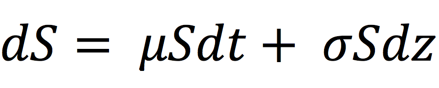
The model is built on several key assumptions such as, the stock price follows a geometric Brownian motion with constant drift and volatility, no arbitrage opportunities, constant risk-free interest rate and options are European-style (options that can only be exercised at maturity).

Key Parameters

In the BSM model, there are five essential parameters to compute the theoretical value of a European-style option is calculated are:

• Strike price (K): fixed price specified in an option contract at which the option holder can buy (for a call) or sell (for a put) the underlying asset if the option is exercised.
• Time to expiration (T): time left until the option expires.
• Current underlying price (S₀): the market price of underlying asset (commodities, precious metals like gold, currencies, bonds, etc.).
• Risk-free interest rate (r): the theoretical rate of return on an investment that is continuously compounded per annum.
• Volatility (σ): standard deviation of the returns of the underlying asset.

The strike price (exercise price) and time to expiration (maturity) correspond to characteristics of the option while the current underlying asset price, the risk-free interest rate, and volatility reflect market conditions.

Option payoff

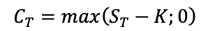
The payoff for a call option gives the value of the option at the moment it expires (T) and is given by the expression below:

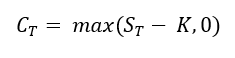
Where C_T is the call option value at expiration, S_T the price of the underlying asset at expiration, and K is the strike price (exercise price) of the option.

Figure 1 below illustrates the payoff function described above for a European-style call option. The example considers a European call written on the S&P 500 index, with a strike price of $5,000 and a time to maturity of 30 days.

Figure 1. Payoff value as a function of the underlying asset price.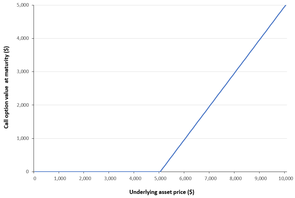

Source: computation by the author.

Call option value

While the value of an option is known at maturity (being determined by its payoff function), its value at any earlier time prior to maturity, and in particular at issuance, is not directly observable. Consequently, a valuation model is required to determine the option’s price at those earlier dates.

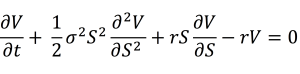
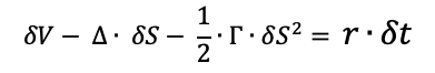
The Black–Scholes–Merton model is formulated as a stochastic partial differential equation and the solution to the partial differential equation (PDE) gives the BSM formula for the value of the option.

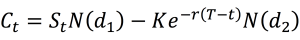
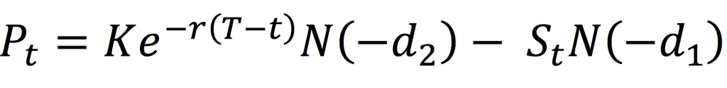
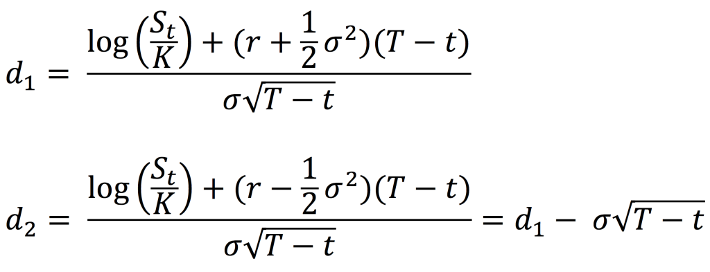
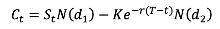
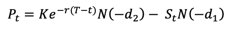
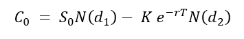
For a European-style call option, the call option value at issuance is given by the following formula:

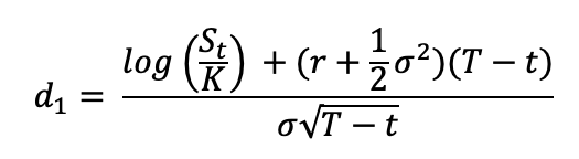
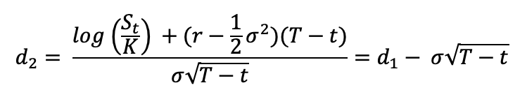
with

Where the notations are as follows:

• C₀= Call option value at issuance (time 0) based on the Black-Scholes-Merton model
• K = Strike price (exercise price)
• T = Time to expiration
• S₀ = Current underlying price (time 0)
• r = Risk-free interest rate
• σ = Volatility of the underlying asset returns
• N(·) = Cumulative distribution function of the standard normal distribution

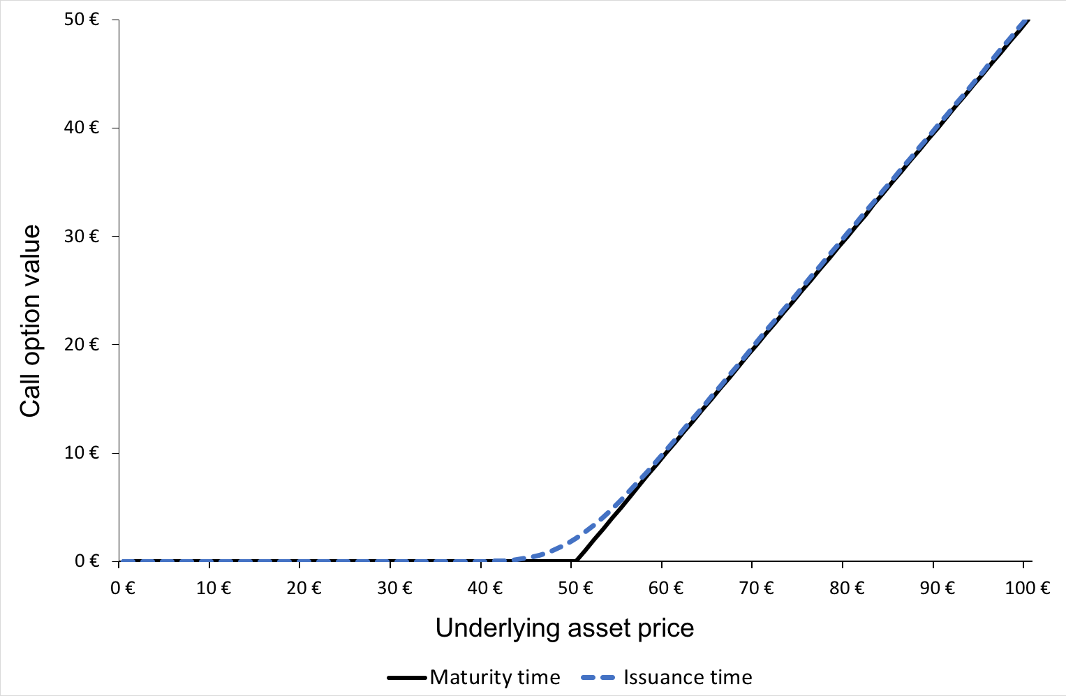
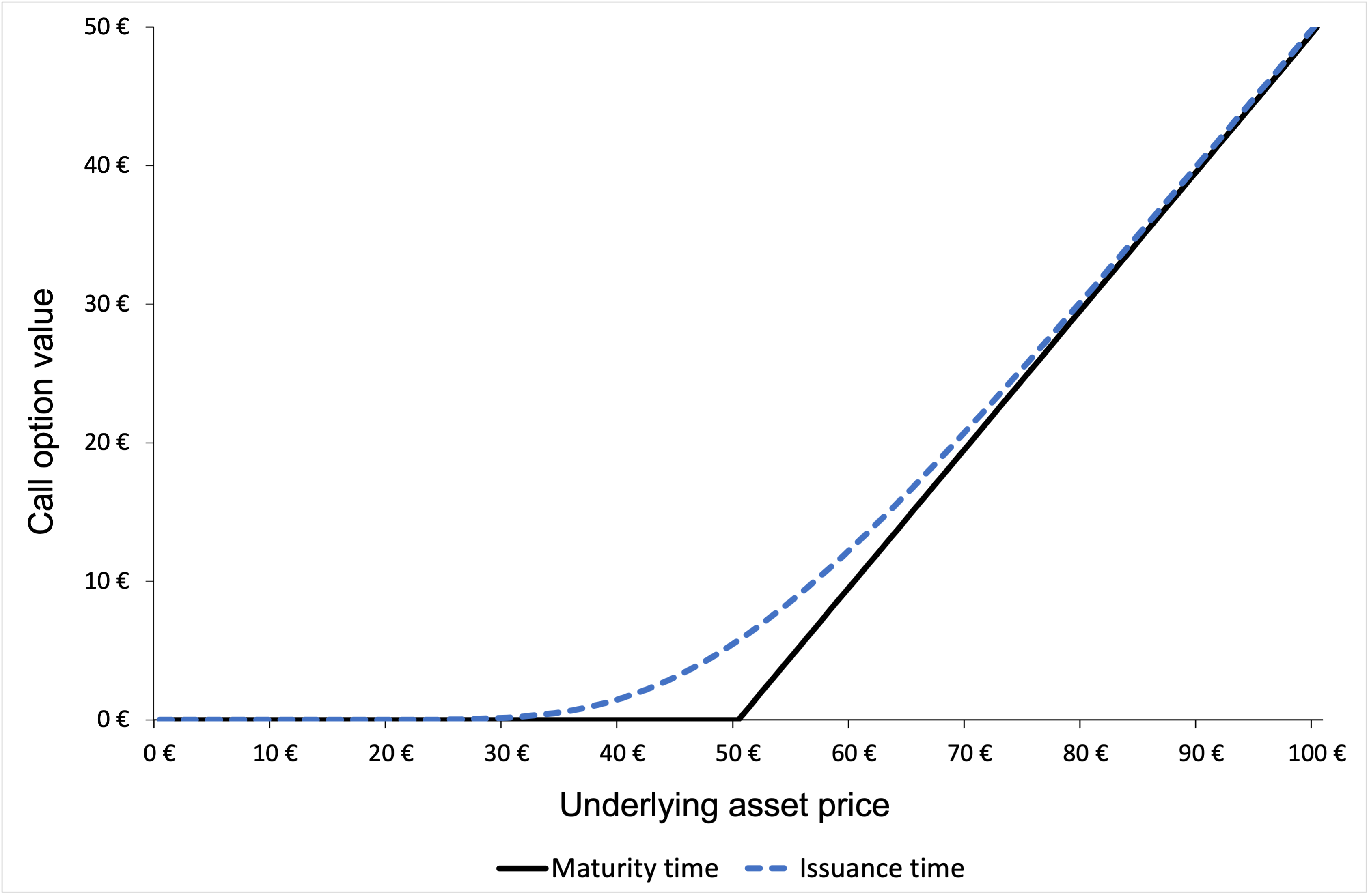
Figure 2 below illustrates the call option value as a function of the underlying asset price. The example considers a European call written on the S&P 500 index, with a strike price of $5,000 and a time to maturity of 30 days. The current price of the underlying index is $6,000, and the risk-free interest rate is set at 3.79% corresponding to the 1-month U.S. Treasury yield, and the volatility is assumed to be 15%.

Figure 2. Call option value as a function of the underlying asset price.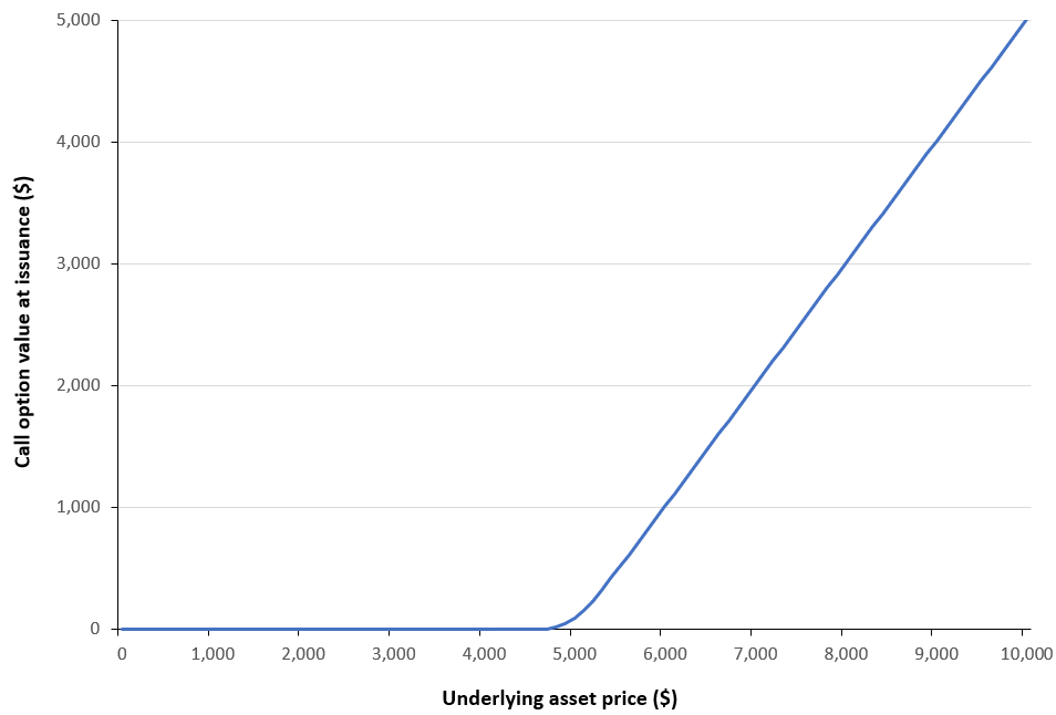

Source: computation by the author (BSM model).

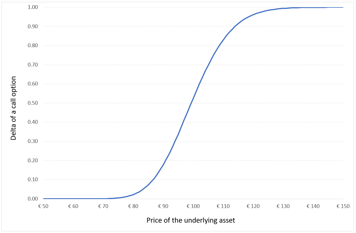
Option and volatility

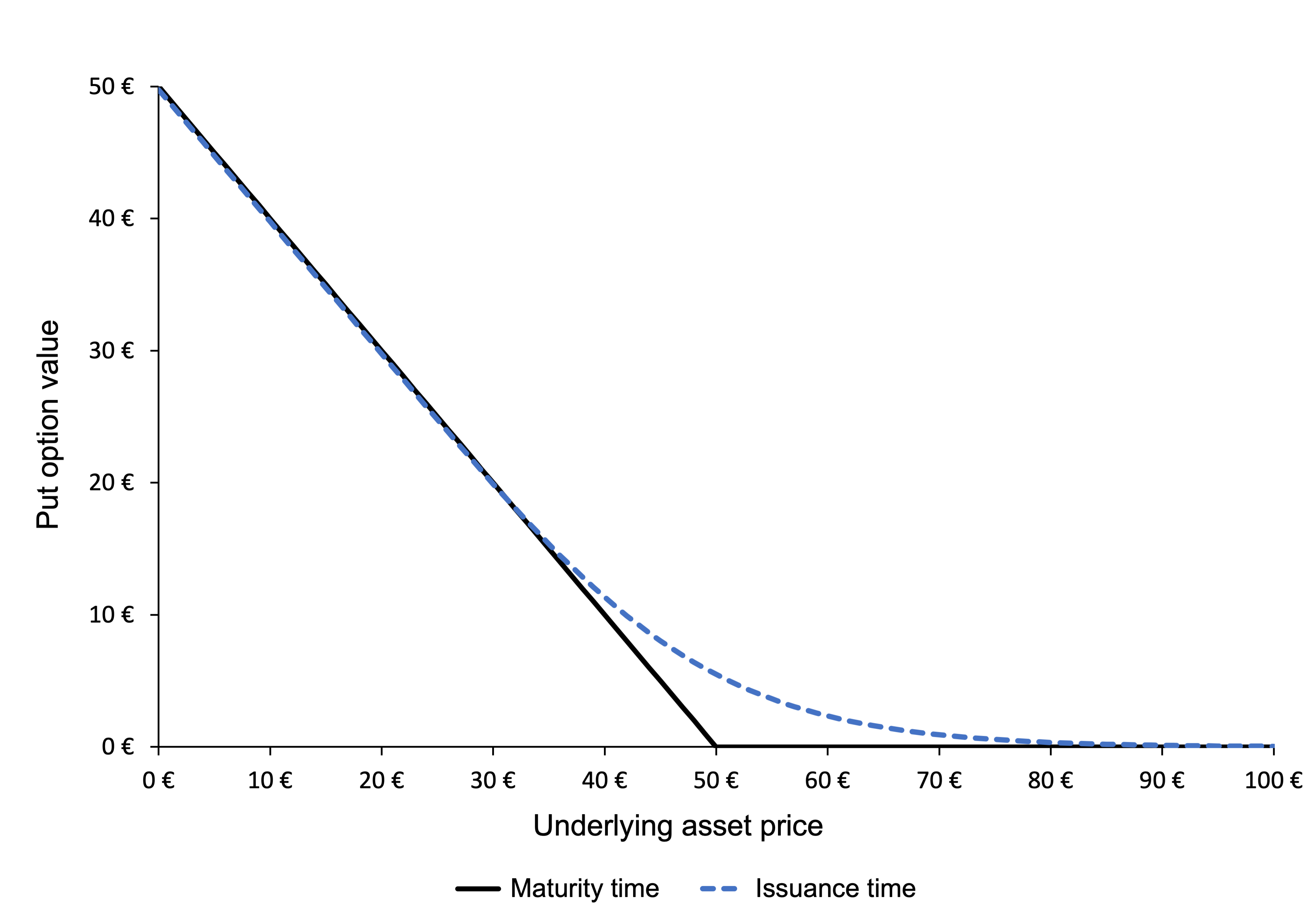
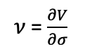
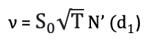
In the Black–Scholes–Merton model, the value of a European call or put option is a monotonically increasing function of volatility. Higher volatility increases the probability of finishing in-the-money while losses remain limited to the option premium, resulting in a strictly positive vega (the first derivative of the option value with respect to volatility) for both calls and puts.

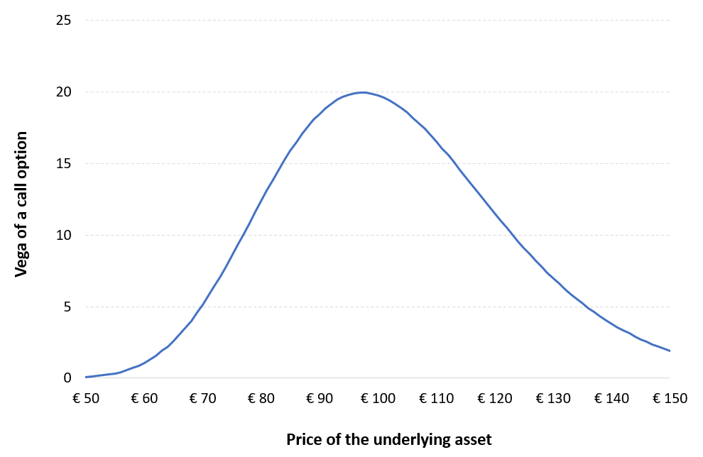
As volatility approaches zero, the option value converges to its intrinsic value, forming a lower bound. With increasing volatility, option values rise toward a finite upper bound equal to the underlying price for calls (and bounded by the strike for puts). An inflection point occurs where volga (the second derivative of the option value with respect to volatility) changes sign: at this point vega is maximized (at-the-money) and declines as the option becomes deep in- or out-of-the-money or as time to maturity decreases.

The upper limit and the lower limit for the call option value function is given below (Hull, 2015, Chapter 11).

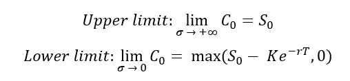
Figure 3 below illustrates the value of a European call option as a function of the underlying asset’s price volatility. The example considers a European call written on the S&P 500 index, with a strike price of $5,000 and a time to maturity of 30 days. The current price of the underlying index is $6,000, and the risk-free interest rate is set at 3.79% corresponding to the 1-month U.S. Treasury yield. A deliberately wide (and economically unrealistic) range of volatility values is employed in order to highlight the theoretical limits of option prices: as volatility tends to infinity, the option value converges to an upper bound ($6,000 in our example), while as volatility approaches zero, the option value converges to a lower bound $1,015.51).

Figure 3. Call option value as a function of price volatility

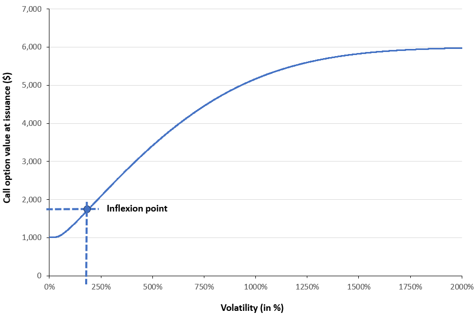
Source: computation by the author (BSM model).

Volatility: the unobservable parameter of the model

When we think of options, the basic equation to remember is “Option = Volatility”. Unlike stocks or bonds, options are not primarily quoted in monetary units (dollars or euros), but rather in terms of implied volatility, expressed as a percentage.

Volatility is not directly observable in financial markets. It is an unobservable (latent) parameter of the pricing model, inferred endogenously from observed option prices through an inversion of the valuation formula given by the BSM model. As a result, option markets are best interpreted as markets for volatility rather than markets for prices.

Out of the five essential parameters of the Black-Scholes-Merton model listed above, the volatility parameter is the unobservable parameter as it is the future fluctuation in price of the underlying asset over the remaining life of the option from the time of observation. Since future volatility cannot be directly observed, practitioners use the inverse of the BSM model to estimate the market’s expectation of this volatility from option market prices, referred to as implied volatility.

Implied Volatility

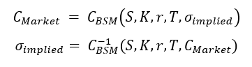
In practice, implied volatility is the volatility parameter that when input into the Black-Scholes-Merton formula yields the market price of the option and represents the market’s expectation of future volatility.

Calculating Implied volatility

The BSM model maps five input variables (S, K, r, T, σ_implied) to a single output variable uniquely: the call option value (Price), such that it’s a bijective function. When the market call option price (C_BSM) is known, we invert this relationship using (S, K, r, T, C_BSM) as inputs to solve for the implied volatility, σ_implied.

Newton-Raphson Method

As there is no closed form solution to calculate implied volatility from the market price, we need a numerical method such as the Newton–Raphson method to compute it. This involves finding the volatility for which the Black–Scholes–Merton option value C_BSM equals the observed market option price C_Market.

We define the function f as the difference between the call option value given by the BSM model and the observed market price of the call option:

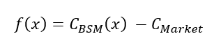
Where x represents the unknown variable (implied volatility) to find and C_Market is considered as a constant in the Newton–Raphson method.

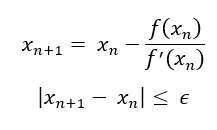
Using the Newton-Raphson method, we can iteratively estimate the root of the function, until the difference between two consecutive estimations is less than the tolerance level (ε).

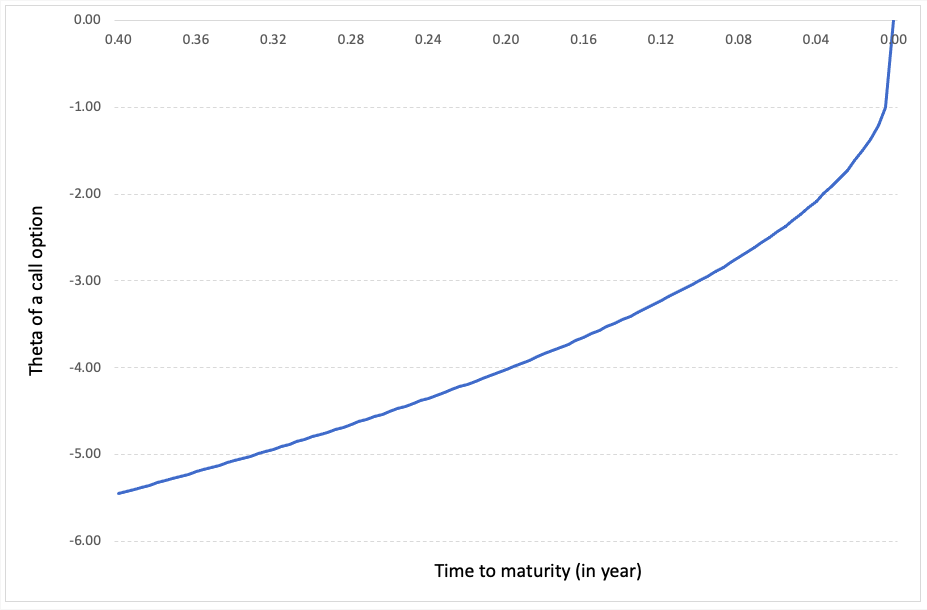
In practice, the inflexion point (Tankov, 2006) is taken as the initial guess, because the function f(x) is monotonic, so for very large or very small initial values, the derivative becomes extremely small (see Figure 3), causing the Newton–Raphson update step to overshoot the root and potentially diverge. Selecting the inflection point also minimizes approximation error, as the second derivative of the function at this point is approximately zero, while the first derivative remains non-zero.

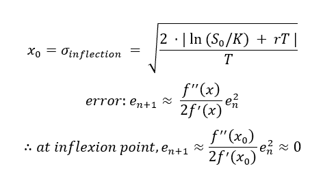
Where σ_inflection is the volatility at the inflection point.

Figure 4 below illustrates how implied volatility varies with the call option price for different values of the market price (computed using the Newton–Raphson method). As before, the example considers a European call written on the S&P 500 index, with a strike price of $5,000 and a time to maturity of 30 days. The current level of the underlying index is $6,000, and the risk-free interest rate is set at 3.79% corresponding to the 1-month U.S. Treasury yield.

Figure 4. Implied volatility vs. Call Option value

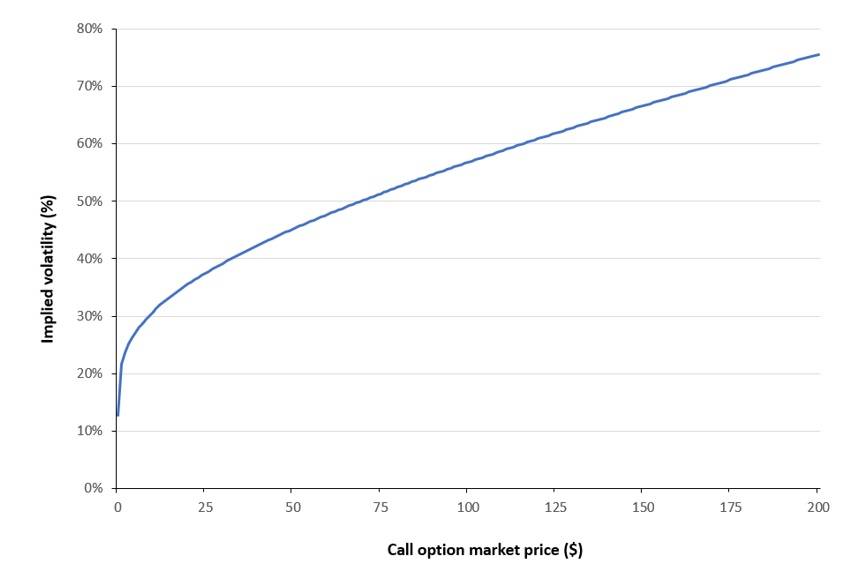
Source: computation by the author.

You can download the Excel file provided below, which contains the calculations and charts illustrating the payoff function, the option price as a function of the underlying asset’s price, the option price as a function of volatility, and the implied volatility as a function of the option price.

You can download the Python code provided below, to calculate the price of a European-style call or put option and calculate the implied volatility from the option market price (BSM model). The Python code uses several libraries.

Alternatively, you can download the R code below with the same functionality as in the Python file.

Why should I be interested in this post?

The seminal Black–Scholes–Merton model was originally developed to price European options. Over time, it has been extended to accommodate a wide range of derivatives, including those based on currencies, commodities, and dividend-paying stocks. As a result, the model is of fundamental importance for anyone seeking to understand the derivatives market and to compute implied volatility as a measure of risk.

Related posts on the SimTrade blog

   ▶ Akshit GUPTA Options

   ▶ Jayati WALIA Black-Scholes-Merton Option Pricing Model

   ▶ Jayati WALIA Implied Volatility

   ▶ Akshit GUPTA Option Greeks – Vega

Useful resources

Academic research

Black F. and M. Scholes (1973) The pricing of options and corporate liabilities. Journal of Political Economy, 81(3), 637–654.

Merton R.C. (1973) Theory of rational option pricing. The Bell Journal of Economics and Management Science, 4(1), 141–183.

Hull J.C. (2022) Options, Futures, and Other Derivatives, 11th Global Edition, Chapter 15 – The Black–Scholes–Merton model, 338–365.

Cox J.C. and M. Rubinstein (1985) Options Markets, First Edition, Chapter 5 – An Exact Option Pricing Formula, 165-252.

Tankov P. (2006) Calibration de Modèles et Couverture de Produits Dérivés (Model calibration and derivatives hedging), Working Paper, Université Paris-Diderot. Available at https://cel.hal.science/cel-00664993/document.

About the BSM model

The Nobel Prize Sveriges Riksbank Prize in Economic Sciences in Memory of Alfred Nobel 1997

Harvard Business School Option Pricing in Theory & Practice: The Nobel Prize Research of Robert C. Merton

Other

NYU Stern Volatility Lab Volatility analysis documentation.

About the author

The article was written in December 2025 by Saral BINDAL (Indian Institute of Technology Kharagpur, Metallurgical and Materials Engineering, 2024-2028 & Research assistant at ESSEC Business School).

   ▶ Discover all articles written by Saral BINDAL