In this article, Snehasish CHINARA (ESSEC Business School, Grande Ecole Program – Master in Management, 2022-2025) explores the academic evolution of capital structure theory, focusing on the delicate balance between debt and equity financing. Starting from the foundational Modigliani and Miller propositions, this post delves into how the introduction of real-world frictions—particularly bankruptcy costs and financial distress—gave rise to the Trade-Off Theory.
Introduction to Capital Structure
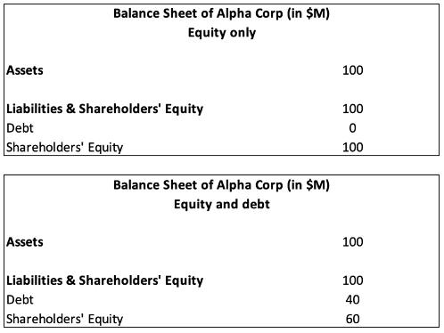
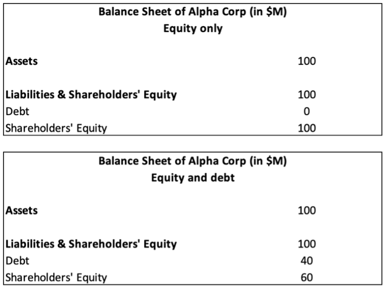
Capital structure refers to the mix of debt and equity financing that a company uses to fund its operations and growth. It is a critical component of corporate finance, as it directly impacts a firm’s cost of capital, financial risk, and overall valuation.
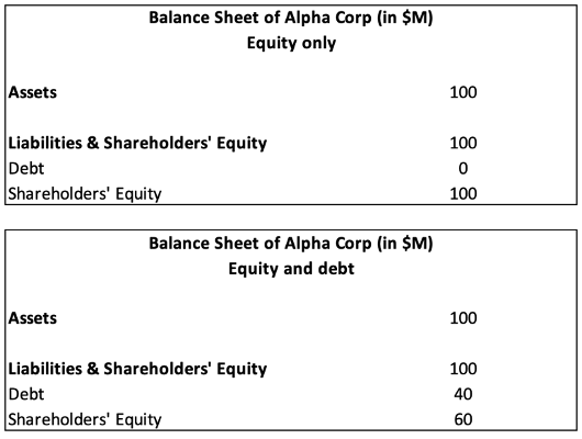
Capital structure is reflected in a company’s balance sheet, which provides a snapshot of its financial position at a given point in time. Specifically, it is composed of two primary financing sources:
1. Debt (Liabilities) – Found under the Liabilities section, debt includes short-term borrowings, long-term loans, bonds payable, and lease obligations. Debt financing requires periodic interest payments and repayment of principal, increasing financial obligations but also benefiting from potential tax shields.
2.Equity (Shareholders’ Equity) – Located under the Shareholders’ Equity section, equity includes common stock, preferred stock, retained earnings, and additional paid-in capital. Equity financing does not require fixed interest payments but dilutes ownership among shareholders.
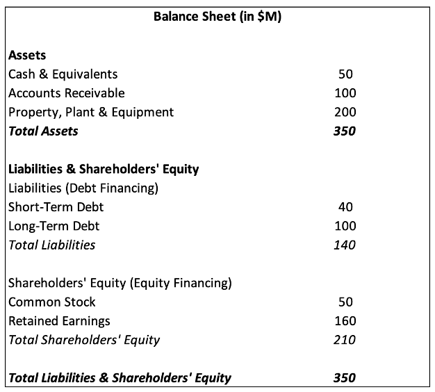
Table 1 below gives a simplified version of a balance sheet.
Table 1 – Simplified Balance Sheet Example

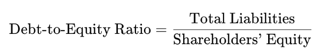
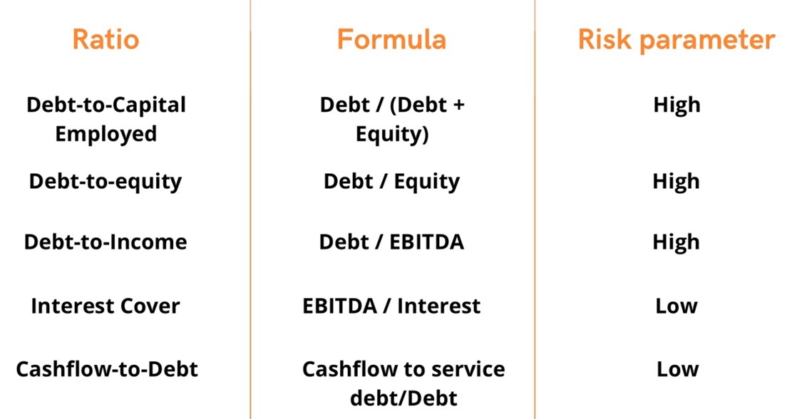
Table 1 shows that the firm finances its $350M in assets with $140M in debt (40%) and $210M in equity (60%), demonstrating a debt-to-equity ratio of 0.67 (=140/210). Additionally, the debt ratio, D/(D+E), measures the proportion of total financing that comes from debt 40% (=140/(140+210)). This indicates that a significant portion of capital is funded through borrowed money, allowing the company to take advantage of the use of debt, but also exposing it to higher financial risk if it faces difficulties in meeting debt obligations. These ratios are a few key indicators used to assess a company’s financial leverage and risk exposure.
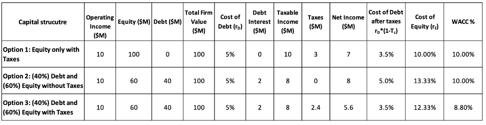
Beyond Taxes — The Real-World Cost of Debt
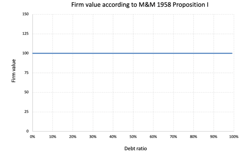
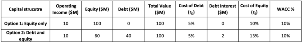
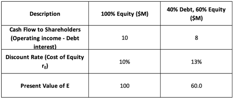
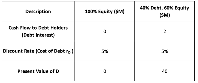
Capital structure theory begins with Modigliani and Miller (1958), who argued that in a perfect market—with no taxes or distress costs—a firm’s value is unaffected by its mix of debt and equity. This implies that financing decisions are irrelevant: the firm’s cost of capital remains unchanged regardless of leverage.
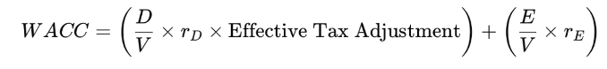
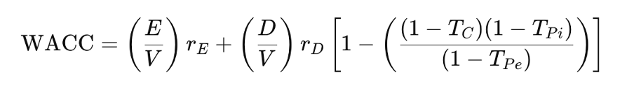
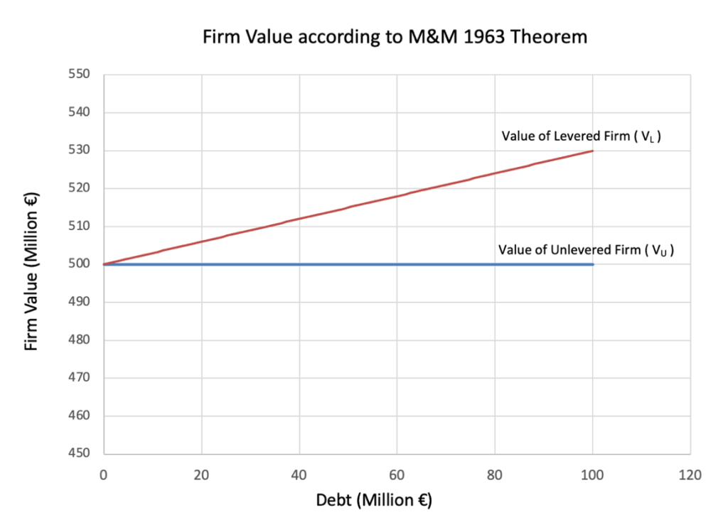
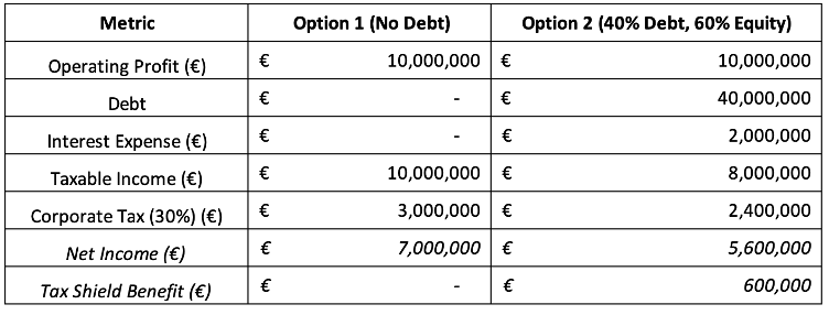
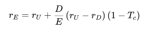
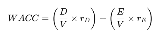
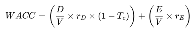
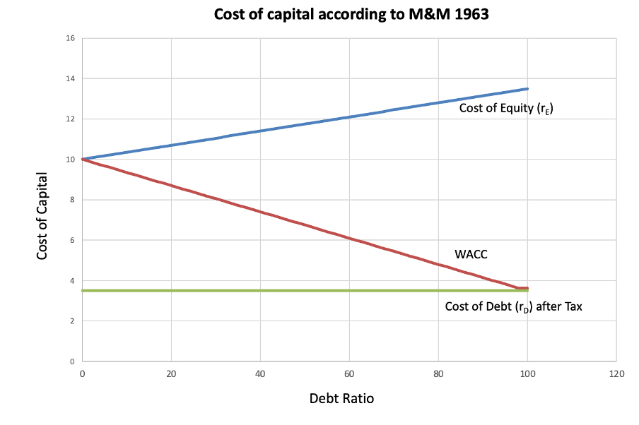
Their later work in 1963 introduced corporate taxes, shifting the narrative. Since interest is tax-deductible, debt creates a tax shield that reduces taxable income, lowering the firm’s WACC and increasing its value. In theory, this would mean the more debt a firm uses, the better.
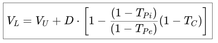
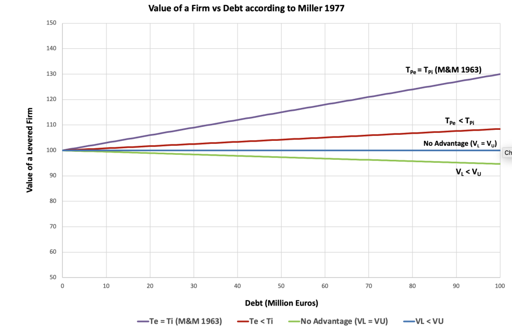
However, this doesn’t match real-world behaviour. Firms rarely use excessive debt. To explain this, Miller (1977) brought personal taxes into the picture. While firms benefit from interest deductibility, investors may face higher taxes on interest income compared to equity income. This reduces the net benefit of debt. At the market level, an equilibrium emerges where additional debt offers no further advantage—explaining why firms stop before 100% leverage.
Together, M&M and Miller show why debt can be attractive due to tax savings—but they don’t account for the costs of debt, which are crucial in practice. This article now turns to academic perspectives that build on these theories by introducing bankruptcy costs, financial distress, and agency issues, offering a more complete view of how firms decide on an optimal capital structure.
The Trade-Off Theory: Balancing Tax Shields and Bankruptcy Costs
While M&M (1963) and Miller (1977) emphasize the tax advantages of debt, real-world firms don’t pursue unlimited leverage. Why? Because with higher debt comes higher financial risk. This leads to the Trade-Off Theory—a more realistic and widely taught framework in modern corporate finance.
At the heart of this theory lies a simple question: How much debt is too much?
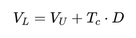
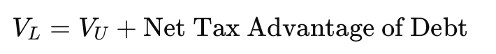
The Trade-Off Theory proposes that firms weigh the benefits of debt (primarily the interest tax shield) against the costs of debt (most notably bankruptcy risk and financial distress costs). The optimal capital structure is achieved when the marginal benefit of taking on more debt equals its marginal cost. Therefore, firms pick capital structure by trading off the benefits of the tax shield from debt against the costs of financial distress (including agency costs of debt).
This framework leads to a simple but powerful relationship:

where:
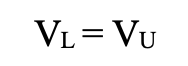
- VL is the value of a levered firm using debt.
- VU is the value of a unlevered firm not using debt but only equity
- Tax shield benefits: arising from the tax deductibility of interest payments
- Expected bankruptcy cost: a function of both the probability of distress and the magnitude of associated losses (probability of distress x cost if distress occurs)
The Trade-Off Theory argues that the value of a firm initially increases with debt due to tax savings from interest deductibility, but only up to a point. Beyond that, the probability of bankruptcy and the costs associated with financial distress begin to outweigh the benefits of the tax shield. Due to this, there exists an optimal capital structure where the marginal benefit of debt exactly equals its marginal cost.
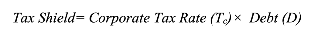
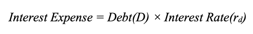
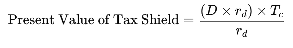
Tax shield benefit: This term represents the annual tax saving due to deductible interest.
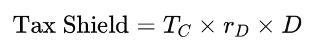
where:
- TC: Corporate tax rate
- rD: Interest rate on debt
- D is the amount of debt of the firm
Expected Bankruptcy Cost:

This cost includes:
- Direct costs (legal, administrative): typically 2–5% of firm value
- Indirect costs (reputation, supplier reactions, customer attrition): potentially far higher
How Firm Value Changes with Debt
According to the Trade-off Theory, the total value of a levered firm equals the value of the firm without leverage plus the present value of the expected tax savings from debt, less the present value of the expected financial distress costs.
It is represented as follows:

where:
- VL is the value of a levered firm using debt.
- VU is the value of a unlevered firm not using debt but only equity
Firms should increase leverage until they reach the optimal level where the firm value (and the net benefit of debt) is maximized. At the optimal leverage, the marginal benefits of interest tax shields that result from increasing leverage are perfectly offset by the marginal costs of financial distress.
Figure 1 – Trade-Off Theory Optimal Leverage
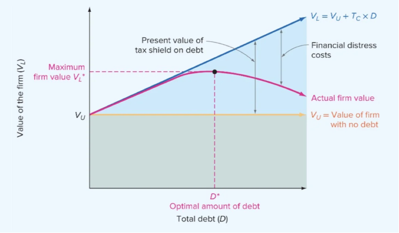
Source: “The Static Theory of Capital Structure” Brealey, Myers, & Allen
Figure 1 above illustrates the Trade-Off Theory of capital structure, which posits that a firm’s value is influenced by two opposing forces: the benefits of debt and the costs of financial distress.
- The upward-sloping blue line represents the firm’s value if we consider only the corporate tax advantage of debt, where each additional unit of debt increases firm value by the present value of the tax shield (Tc×D). However, this idealized trajectory (as per M&M 1963) does not account for real-world frictions.
- As leverage rises, so too does the probability of financial distress, bringing with it both direct costs (legal and administrative expenses) and indirect costs (reputation damage, lost sales, supplier concerns). These rising costs are reflected by the gap between the blue and pink curves.
- The pink curve represents the actual value of a levered firm after subtracting distress costs. It shows the actual value of the firm once these financial distress costs are taken into account. Initially, this curve rises along with the tax shield benefits. But after a certain point, the marginal cost of debt begins to exceed its marginal benefit, causing the curve to flatten and then decline.
- The pink curve peaks at the point marked D∗—the firm’s optimal capital structure. The point D∗ is the optimal amount of debt where the marginal benefit of the tax shield is exactly offset by the marginal expected cost of financial distress.
- To the left of D∗, adding more debt increases firm value; to the right of it, further leverage diminishes value. The curve therefore reflects a concave relationship between debt and firm value, with the maximum point corresponding to the firm’s optimal capital structure.
- Leverage is a double-edged sword—it creates value through tax savings but erodes it through risk.
- The optimal debt level is not universal—it depends on a firm’s industry, asset type, cash flow stability, and access to capital markets.
- Real-world capital structure decisions are about finding a balance, not maximizing one benefit in isolation.
Static vs. Dynamic Trade-Off Models: From Simplified Theory to Real-World Complexity
The traditional Trade-Off Theory provides a powerful intuition: firms balance the benefits of debt (tax shields) against its costs (financial distress). However, how firms actually make capital structure decisions over time is more complex than the simple static view. This brings us to an important academic distinction: static vs. dynamic trade-off models.
Static Trade-Off Models: A Snapshot of Capital Structure
A static trade-off model is a one-period, one-time optimization framework. It assumes that a firm evaluates all its financing options at a single point in time and selects the capital structure that maximizes firm value. The firm is thought to instantly move to its optimal leverage ratio and maintain it indefinitely.
This model gives us a clean formula for firm value:

While this is helpful in teaching and early analysis, it oversimplifies real-world decision-making. Firms don’t reset their debt every day based on a formula. Instead, they must plan, adjust, and adapt—which is where dynamic models offer deeper insight.
Dynamic Trade-Off Models: Capturing Real-World Decision-Making
Dynamic trade-off models build on the static framework by recognizing that:
Capital structure is adjusted over time, not all at once. Firms face adjustment costs when issuing new debt or equity (e.g., flotation costs, signaling effects).
Business conditions, tax environments, interest rates, and risk evolve. Managers are forward-looking—they consider not only current benefits and costs but also future risks, taxes, and financing needs.
In these models, the optimal debt level is not a fixed point. Instead, firms operate within a target range of leverage and make gradual adjustments toward it when the benefits outweigh the costs of doing so.
For example:
A firm may not issue new debt today even if it’s slightly under-leveraged, because issuing comes with costs. It might instead wait for a better interest rate, a tax law change, or an internal cash flow event.
Dynamic models are particularly well-captured in the work of:
- Fischer, Heinkel, and Zechner (1989) – who modelled how firms behave in a stochastic environment where recapitalization is costly.
- Leland (1994) – who showed that default thresholds and optimal leverage depend on firm value and volatility over time.
Types of Bankruptcy Costs: The Hidden Burden of Excessive Leverage
While tax benefits of debt are quantifiable and immediate, the costs of financial distress—especially bankruptcy—are more nuanced, less visible, and often underestimated. These costs are central to the Trade-Off Theory, and understanding their components is essential for evaluating real-world capital structures.
Bankruptcy costs can be broadly classified into three types:
1. Direct Bankruptcy Costs
These are the explicit, out-of-pocket expenses incurred during legal bankruptcy proceedings.
- Legal fees, court costs, bankruptcy consultants
- Administrative expenses, such as auditing and trustee services
Empirical studies suggest that direct costs range from 2–5% of firm value, though they may be higher in complex bankruptcies. While these are easier to measure, they are not necessarily the largest component.
Example: A manufacturing firm with a $500 million valuation that enters Chapter 11 could incur $10–25 million in legal and court-related costs alone.
2. Indirect Bankruptcy Costs
These are opportunity costs or value losses incurred even if bankruptcy does not occur—simply being in distress can harm the business.
- Loss of customers: Buyers lose trust in a distressed brand.
- Supplier tightening: Suppliers demand advance payments or withdraw credit.
- Employee turnover: Top talent exits due to job insecurity.
- Delayed investments: Management focuses on liquidity over strategy.
Indirect costs are often much larger than direct ones—estimated at 10–20% of firm value in some studies.
Example: A hotel chain facing debt pressure may see a fall in bookings, reduced vendor support, and higher staff attrition—impacting operations even before legal proceedings begin.
3. Agency Costs of Debt
As financial distress increases, so do agency conflicts between debt holders and equity holders.
Two prominent issues are:
- Asset Substitution Problem – Shareholders may prefer riskier projects with higher upside (but higher default risk) because they capture the gains, while losses are partially borne by creditors.
- Underinvestment Problem – Highly leveraged firms might pass on positive NPV projects because the gains would go to debt holders, not shareholders. Thus, debt discourages investment when it is most needed.
These agency costs distort management incentives, especially when firms are close to violating debt covenants or already under pressure.
Academic Contributions on Bankruptcy and Alternative Views on Capital Structure
Pecking Order Theory and Information Asymmetry
Contrasting the Trade-Off Theory, Myers and Majluf (1984) introduced the Pecking Order Theory, which prioritizes financing sources based on information asymmetry. Firms prefer internal financing (retained earnings) first, then debt, and issue equity only as a last resort. This hierarchy arises because managers possess more information about the firm’s value than external investors, leading to adverse selection concerns when issuing new equity.
Dynamic Models of Capital Structure
Recognizing that capital structure decisions are not static, researchers have developed dynamic models to reflect real-world complexities. Leland (1994) incorporated factors such as agency costs, taxes, and bankruptcy costs into a continuous-time framework, providing insights into how firms adjust their leverage over time in response to changing conditions.
Human Capital and Bankruptcy Risk
Recent studies have explored the interplay between human capital and capital structure. For instance, research by Berk, Stanton, and Zechner (2010) examines how firms with significant human capital considerations may adopt lower leverage to mitigate the adverse effects of financial distress on their workforce and overall operations.
Empirical Evidence and Contemporary Reviews
Empirical studies have tested these theories across various contexts. For example, research published in the Journal of Finance investigates how bankruptcy risk influences firms’ capital structure choices, revealing an inverse relationship between bankruptcy risk and leverage. Comprehensive literature reviews, such as those by Cerkovskis et al. (2022) and Visinescu and Micuda (2023), provide critical analyses of the evolution and empirical validation of capital structure theories, offering valuable insights for both scholars and practitioners.
Practical Considerations in Capital Structure Decisions
While theories like Modigliani-Miller (M&M), the Trade-Off Theory, and Agency Cost Theory provide useful frameworks for understanding capital structure, real-world evidence shows that firms consider multiple factors beyond theory when making financing decisions. Empirical studies highlight how industries, economic conditions, credit ratings, and market perceptions influence a company’s choice between debt and equity.
Real-World Capital Structure Choices
Empirical research supports the idea that firms do not strictly follow any single capital structure theory but instead balance tax advantages, financial flexibility, and risk. Some key observations from real-world studies include:
- Myers (1984) found that firms follow a “Pecking Order” when raising funds, preferring internal financing (retained earnings) first, followed by debt, and issuing equity as a last resort due to information asymmetry.
- Graham (2000) estimated that firms use only about 60% of the potential tax benefits of debt, indicating that firms hesitate to take on excessive leverage due to bankruptcy risks.
- Frank & Goyal (2009) confirmed that larger, more profitable firms tend to have higher leverage, while smaller, riskier firms avoid debt due to financial distress concerns.
These studies suggest that firms do not maximize leverage, but rather choose a debt level that balances benefits and risks based on firm size, profitability, and market conditions.
Why Should I Be Interested in This Post?
Understanding a firm’s optimal debt structure is essential for anyone involved in finance, strategy, or investment analysis. Whether you’re an investor evaluating risk, a finance professional shaping capital decisions, or a student building foundational knowledge, the trade-off between debt and equity lies at the core of corporate financial strategy. This post offers a deep dive into the academic perspectives on capital structure, highlighting how bankruptcy costs, financial distress, and tax considerations influence real-world financing decisions. By mastering these concepts, you’ll be better equipped to assess firm value, understand risk-return dynamics, and make more informed financial judgments in a world where leverage can both create and destroy value.
Related posts on the SimTrade blog
▶ Snehasish CHINARA Optimal capital structure with corporate and personal taxes: Miller 1977
▶ Snehasish CHINARA Optimal capital structure with taxes: Modigliani and Miller 1963
▶ Snehasish CHINARA Optimal capital structure with no taxes: Modigliani and Miller 1958
▶ Snehasish CHINARA Solvency and Insolvency in the Corporate World
▶ Snehasish CHINARA Illiquidity, Liquidity and Illiquidity in the Corporate World
▶ Snehasish CHINARA Illiquidity, Solvency & Insolvency : A Link to Bankruptcy Procedures
▶ Snehasish CHINARA Chapter 7 vs Chapter 11 Bankruptcies: Insights on the Distinction between Liquidations & Reorganisations
▶ Snehasish CHINARA Chapter 7 Bankruptcies: A Strategic Insight on Liquidations
▶ Snehasish CHINARA Chapter 11 Bankruptcies: A Strategic Insight on Reorganisations
▶ Akshit GUPTA The bankruptcy of Lehman Brothers (2008)
▶ Akshit GUPTA The bankruptcy of the Barings Bank (1996)
▶ Anant JAIN Understanding Debt Ratio & Its Impact On Company Valuation