Systematic risk

Youssef_Louraoui

In this article, Youssef LOURAOUI (Bayes Business School, MSc. Energy, Trade & Finance, 2021-2022) presents the systematic risk of financial assets, a key concept in asset pricing models and investment management theories more generally.

This article is structured as follows: we introduce the concept of systematic risk. We then explain the mathematical foundation of this concept. We present an economic understanding of market risk on recent events.

Portfolio Theory and Risk

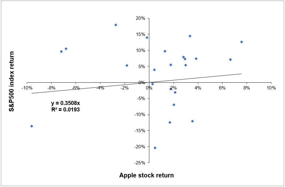
Markowitz (1952) and Sharpe (1964) developed a framework on risk based on their significant work in portfolio theory and capital market theory. All rational profit-maximizing investors seek to possess a diversified portfolio of risky assets, and they borrow or lend to get to a risk level that is compatible with their risk preferences under a set of assumptions. They demonstrated that the key risk measure for an individual asset is its covariance with the market portfolio under these circumstances (the beta).

The fraction of an individual asset’s total variance attributable to the variability of the total market portfolio is referred to as systematic risk, which is assessed by the asset’s covariance with the market portfolio. Systematic risk can be decomposed into the following categories:

Interest rate risk

We are aware that central banks, such as the Federal Reserve, periodically adjust their policy rates in order to boost or decrease the rate of money in circulation in the economy. This has an effect on the interest rates in the economy. When the central bank reduces interest rates, the money supply expands, allowing companies to borrow more and expand, and when the policy rate is raised, the reverse occurs. Because this is cyclical in nature, it cannot be diversified.

Inflation risk

When inflation surpasses a predetermined level, the purchasing power of a particular quantity of money reduces. As a result of the fall in spending and consumption, overall market returns are reduced, resulting in a decline in investment.

Exchange Rate Risk

As the value of a currency reduces in comparison to other currencies, the value of the currency’s returns reduces as well. In such circumstances, all companies that conduct transactions in that currency lose money, and as a result, investors lose money as well.

Geopolitical Risks

When a country has significant geopolitical issues, the country’s companies are impacted. This can be mitigated by investing in multiple countries; but, if a country prohibits foreign investment and the domestic economy is threatened, the entire market of investable securities suffers losses.

Natural disasters

All companies in countries such as Japan that are prone to earthquakes and volcanic eruptions are at risk of such catastrophic calamities.

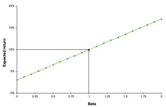
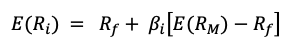
Following the Capital Asset Pricing Model (CAPM), the return on asset i, denoted by Ri can be decomposed as
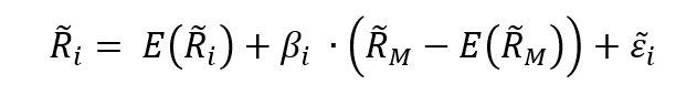
img_SimTrade_return_decomposition

Where:

  • Ri the return of asset i
  • E(Ri) the risk premium of asset i
  • βi the measure of the risk of asset i
  • RM the return of the market
  • E(RM) the risk premium of the market
  • RM – E(RM) the market factor
  • εi represent the specific part of the return of asset i

The three components of the decomposition are the expected return, the market factor and an idiosyncratic component related to asset only. As the expected return is known over the period, there are only two sources of risk: systematic risk (related to the market factor) and specific risk (related to the idiosyncratic component).

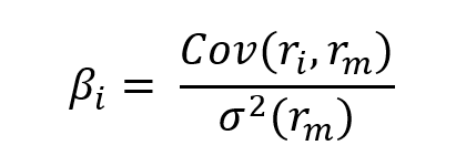
The beta of the asset with the market is computed as:
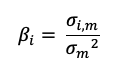
Beta

Where:

  • σi,m : the covariance of the asset return with the market return
  • σm2 : the variance of market return

The total risk of the asset measured by the variance of asset returns can be computed as:
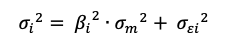
Decomposition of total risk

Where:

  • βi2 * σm2 = systematic risk
  • σεi2 = specific risk

In this decomposition of the total variance, the first component corresponds to the systematic risk and the second component to the specific risk.

Systematic risk analysis in recent times

The volatility chart depicts the evolution of implied volatility for the S&P 500 and US Treasury bonds – the VIX and MOVE indexes, respectively. Implied volatility is the price of future volatility in the option market. Historically, the two markets have been correlated during times of systemic risk, like as in 2008 (Figure 1).

Figure 1. Volatility trough time (VIX and MOVE index).
Volatility trough time (VIX and MOVE index)
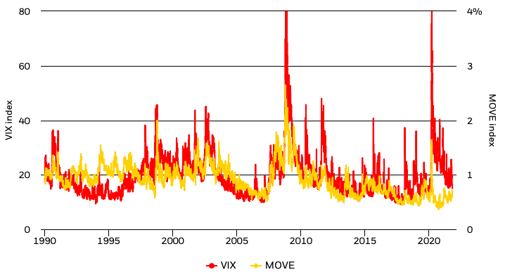
Sources: BlackRock Risk and Quantitative Analysis and BlackRock Investment Institute, with data from Bloomberg and Bank of America Merrill Lynch, October 2021 (BlackRock, 2021).

The VIX index has declined following a spike in September amid the equity market sell-off. It has begun to gradually revert to pre-Covid levels. The periodic, albeit brief, surges throughout the year underscore the underlying fear about what lies beyond the economic recovery and the possibility of a wide variety of outcomes. The MOVE index — a gauge of bond market volatility – has remained relatively stable in recent weeks, despite the rise in US Treasury yields to combat the important monetary policy to combat the effect of the pandemic. This could be a reflection of how central banks’ purchases of government bonds are assisting in containing interest rate volatility and so supporting risk assets (BlackRock, 2021).

The regime map depicts the market risk environment in two dimensions by plotting market risk sentiment and the strength of asset correlations (Figure 2).

Figure 2. Regime map for market risk environment.
Regime map for market risk environment
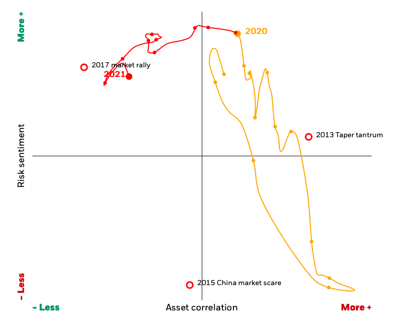
Source: BlackRock Risk and Quantitative Analysis and BlackRock Investment Institute, October 2021 (BlackRock, 2021).

Positive risk sentiment means that riskier assets, such as equities, are outperforming less risky ones. Negative risk sentiment means that higher-risk assets underperform lower-risk assets.

Due to the risk of fast changes in short-term asset correlations, investors may find it challenging to guarantee their portfolios are correctly positioned for the near future. When asset correlation is higher (as indicated by the right side of the regime map), diversification becomes more difficult and risk increases. When asset prices are less correlated (on the left side of the map), investors have greater diversification choices.

When both series – risk sentiment and asset correlation – are steady on the map, projecting risk and return becomes easier. However, when market conditions are unpredictable, forecasting risk and return becomes substantially more difficult. The map indicates that we are still in a low-correlation environment with a high-risk sentiment, which means that investors are rewarded for taking a risk (BlackRock, 2021). In essence, investors should use diversification to reduce the specific risk of their holding coupled with macroeconomic fundamental analysis to capture the global dynamics of the market and better understand the sources of risk.

Why should I be interested in this post?

Market risks fluctuate throughout time, sometimes gradually, but also in some circumstances dramatically. These adjustments typically have a significant impact on the right positioning of a variety of different types of investment portfolios. Investors must walk a fine line between taking enough risks to achieve their objectives and having the proper instruments in place to manage sharp reversals in risk sentiment.

Related posts on the SimTrade blog

   ▶ Louraoui Y. Systematic risk and specific risk

   ▶ Youssef LOURAOUI Specific risk

   ▶ Youssef LOURAOUI Beta

   ▶ Youssef LOURAOUI Portfolio

   ▶ Youssef LOURAOUI Markowitz Modern Portfolio Theory

   ▶ Jayati WALIA Capital Asset Pricing Model (CAPM)

Useful resources

Academic research

Markowitz, H. 1952. Portfolio Selection. The Journal of Finance, 7(1): 77-91.

Mossin, J. 1966. Equilibrium in a Capital Asset Market. Econometrica, 34(4): 768-783.

Sharpe, W.F. 1963. A Simplified Model for Portfolio Analysis. Management Science, 9(2): 277-293.

Sharpe, W.F. 1964. Capital Asset Prices: A Theory of Market Equilibrium under Conditions of Risk. The Journal of Finance, 19(3): 425-442.

Business analysis

BlackRock, 2021. Market risk monitor

About the author

The article was written in April 2022 by Youssef LOURAOUI (Bayes Business School, MSc. Energy, Trade & Finance, 2021-2022).

Beta

Youssef_Louraoui

In this article, Youssef LOURAOUI (Bayes Business School, MSc. Energy, Trade & Finance, 2021-2022) explains the concept of beta, one of the most fundamental concepts in the financial industry, which is heavily used in asset management to assess the risk of assets and portfolios.

This article is structured as follows: we introduce the concept of beta in asset management. Next, we present the mathematical foundations of the concept. We finish with an interpretation of beta values for risk analysis.

Introduction

The (market) beta represents the sensitivity of an individual asset or a portfolio to the fluctuations of the market. This risk measure helps investors to predict the movements of their assets according to the movements of the market overall. It measures the asset risk in comparison with the systematic risk inherent to the market.

In practice, the beta for a portfolio (fund) in respect to the market M represented by a predefined index (the S&P 500 index for example) indicates the fund’s sensitivity to the index. Essentially, the fund’s beta to the index attempts to capture the amount of money made (or lost) when the index increases (or decreases) by a specified amount.

Graphically, the beta represents the slope of the straight line through a regression of data points between the asset return in comparison to the market return for different time periods. It is a traditional risk measure used in the asset management industry. To give a more insightful explanation, a regression analysis has been performed using data for the Apple stock (APPL) and the S&P500 index to see how the stock behaves in relation to the market fluctuations (monthly data for the period July 2018 – June 2020). Figure 1 depicts the regression between Apple stock and the S&P500 index (excess) returns. The estimated beta is between zero and one (beta = 0.3508), which indicates that the stock price fluctuates less than the market index.

Figure 1. Linear regression of the Apple stock return on the S&P500 index return.
Beta analysis for Apple stock return
Source: Computation by the author (data source: Thomson Reuters).

Mathematical derivation of Beta

Use of beta

William Sharpe, John Lintner, and Jan Mossin separately developed key capital markets theory as a result of Markowitz’s previous works: the Capital Asset Pricing Model (CAPM). The CAPM was a huge evolutionary step forward in capital market equilibrium theory since it enabled investors to appropriately value assets in terms of systematic risk, defined as the market risk which cannot be neutralized by the effect of diversification.

The CAPM expresses the expected return of an asset a function of the risk-free rate, the beta of the asset, and the expected return of the market. The main result of the CAPM is a simple mathematical formula that links the expected return of an asset to these different components. For an asset i, it is given by:

CAPM risk beta relation

Where:

  • E(ri) represents the expected return of asset i
  • rf the risk-free rate
  • βi the measure of the risk of asset i
  • E(rm) the expected return of the market
  • E(rm)- rf the market risk premium.

The risk premium for asset i is equal to βi(E(rm)- rf), that is the beta of asset i, βi, multiplied by the risk premium for the market, E(rm)- rf.

In this model, the beta (β) parameter is a key parameter and is defined as:

CAPM beta formula

Where:

  • Cov(ri, rm) represents the covariance of the return of asset i with the return of the market
  • σ2(rm) the variance of the return of the market.

Excel file to compute the beta

You can download below an Excel file with data for Apple stock returns and the S&P500 index returns (used as a representation of the market). This Excel file computes the beta of apple with the S&P500 index.

Download the Excel file to estimate the beta of Apple stock

Interpretation of the beta

Beta helps investors to explain how the asset moves compared to the market. More specifically, we can consider the following cases for beta values:

  • β = 1 indicates a fluctuation between the asset and its benchmark, thus the asset tends to move at a similar rate than the market fluctuations. A passive ETF replicating an index will present a beta close to 1 with its associated index.
  • 0 < β < 1 indicates that the asset moves at a slower rate than market fluctuations. Defensive stocks, stocks that deliver consistent returns without regarding the market state like P&G or Coca Cola in the US, tend to have a beta with the market lower than 1.
  • β > 1 indicates a more aggressive effect of amplification between the asset price movements with the market movements. Call options tend to have higher betas than their underlying asset.
  • β = 0 indicates that the asset or portfolio is uncorrelated to the market. Govies, or sovereign debt bonds, tend to have a beta-neutral exposure to the market.
  • β < 0 indicates an inverse effect of market fluctuation impact in the asset volatility. In this sense, the asset would behave inversely in terms of volatility compared to the market movements. Put options and Gold typically tend to have negative betas.

Why should I be interested in this post?

If you are a business school or university student, this post will help you to understand the fundamentals of investment.

Related posts on the SimTrade blog

   ▶ Youssef LOURAOUI Systematic and specific risks

   ▶ Youssef LOURAOUI Portfolio

   ▶ Youssef LOURAOUI Alpha

   ▶ Jayati WALIA Capital Asset Pricing Model (CAPM)

Useful resources

Academic research

Fama, Eugene F. 1965. The Behavior of Stock Market Prices.Journal of Business 37: January 1965, 34-105.

Fama, Eugene F. 1967. Risk, Return, and General Equilibrium in a Stable Paretian Market. Chicago, IL: University of Chicago.Unpublished manuscript.

Fama, Eugene F. 1968. Risk, Return, and Equilibrium: Some Clarifying Comments. Journal of Finance, (23), 29-40.

Lintner, J. 1965a. The Valuation of Risk Assets and the Selection of Risky Investments in Stock Portfolios and Capital Budgets. The Review of Economics and Statistics 47(1): 13-37.

Lintner, J. 1965b. Security Prices, Risk and Maximal Gains from Diversification. The Journal of Finance 20(4): 587-615.

Mangram, M.E., 2013. A simplified perspective of the Markowitz Portfolio Theory. Global Journal of Business Research, 7(1): 59-70.

Markowitz, H., 1952. Portfolio Selection. The Journal of Finance, 7(1): 77-91.

Mossin, J. 1966. Equilibrium in a Capital Asset Market. Econometrica 34(4): 768-783.

Sharpe, W.F. 1963. A Simplified Model for Portfolio Analysis. Management Science 9(2): 277-293.

Sharpe, W.F. 1964. Capital Asset Prices: A Theory of Market Equilibrium under Conditions of Risk. The Journal of Finance 19(3): 425-442.

Business analysis

JP Morgan Asset Management, 2021. Glossary of investment terms: Beta

Man Institute, 2021. How to calculate the Beta of a portfolio to a factor

Nasdaq, 2021. Beta

About the author

The article was written in November 2021 by Youssef LOURAOUI (Bayes Business School, MSc. Energy, Trade & Finance, 2021-2022).

Security Market Line (SML)

Youssef_Louraoui

In this article, Youssef LOURAOUI (Bayes Business School, MSc. Energy, Trade & Finance, 2021-2022) presents the Security Market Line (SML), a key concept in asset pricing derived from the Capital Asset Pricing Model (CAPM).

This article is structured as follows: we first introduce the concept of Security Market Line (SML). We then present the mathematical foundations of the SML. We finish by presenting an investment strategy that can be implemented relying on the SML.

Security Market Line

The SML reflects the risk-return combinations accessible in the capital market at any given time for all risky assets. Investors would choose investments based on their risk appetites; some would only consider low-risk investments, while others would welcome high-risk investments. The SML is derived from the Capital Asset Pricing Model (CAPM), which describes the trade-off between risk and expected return for efficient portfolios.

The expected relationship between risk and return is depicted in Figure 1. It demonstrates that as perceived risk increases, investors’ required rates of return increase.

Figure 1. Security Market Line.
Security Market Line
Source: Computation by the author.

Under the CAPM framework, all investors will choose a position on the capital market line by borrowing or lending at the risk-free rate, since this maximizes the return for a given level of risk. Whereas the CML indicates the rates of return of a specific portfolio, the SML represents the risk and return of the market at a given point in time and indicates the expected returns of individual assets. Also, while the measure of risk in the CML is the standard deviation of returns (total risk), the measure of risk in the SML is the systematic risk, or beta. Figure 2 depicts the SML line combined with four different assets. Asset A and B are above the SML line, which implies that they are overvalued. Asset C and D are below the SML which implies that they are undervalued. From Figure 2, we can implement an investment strategy by going long if the asset or portfolio lies under the SML and going short if the asset or portfolio is greater than the SML.

Figure 2. Security Market Line with a plot of different assets.
Security Market Line with a plot of different assets
Source: Computation by the author.

Mathematical foundation

The SML plots an individual security’s expected rate of return against systematic, undiversifiable risk. The risk associated with an individual risky security is determined by the volatility of the security’s return, not by the market portfolio’s return. Individual risky securities bear a proportional share of the systematic risk. The only risk that an investor should be compensated for is systematic risk, which cannot be neutralized through diversification. This risk is quantified using the beta, which refers to a security’s sensitivity to market fluctuations. The slope of the SML is equal to the market risk premium and reflects the risk-reward trade-off at a particular point in time. We can define the line of the SML as:

img_SimTrade_SML_graph

Mathematically, we can deconstruct the SML as:

SML_formula

Where

  • E(Ri) represents the expected return of asset i
  • Rf is the risk-free interest rate
  • βi measures the systematic risk of asset i
  • E(RM) represents the expected return of the market
  • E[RM – Rf] represents the market risk premium.

Beta and the market factor

William Sharpe (1964), John Lintner (1965), and Jan Mossin (1966) independently developed the Capital Asset Pricing Model (CAPM). The CAPM was a significant evolutionary step forward in capital market equilibrium theory because it allowed investors to value assets correctly in terms of risk. The CAPM makes a distinction between two forms of risk: systematic and specific risk. Systematic risk refers to the risk posed by the market’s basic structure, its participants, and all non-diversifiable elements such as monetary policy, political events, and natural disasters. By contrast, specific risk refers to the risk inherent in a particular asset and so is diversifiable. As a result, the CAPM solely captures systematic risk via the beta measure, with the market’s beta equal to one, lower-risk assets having a beta less than one, and higher-risk assets having a beta larger than one.

In the late 1970s, the portfolio management industry sought to replicate the market portfolio return, but as financial research advanced and significant contributions were made, it enabled the development of additional factor characteristics to capture additional performance. This resulted in the development of what is now known as factor investing.

Estimation of the Security Market Line

You can download an Excel file with data to estimate the Security Market Line.

Download the Excel file to compute the Security Market Line

Why should I be interested in this post?

The security market line is frequently used by portfolio managers and investors to determine the suitability of an investment product for inclusion in a portfolio. The SML is useful for determining whether a security’s expected return is favourable in comparison to its level of risk. The SML is frequently used to compare two similar securities that offer approximately the same rate of return to determine which one has the lowest inherent market risk in relation to the expected rate of return. Additionally, the SML can be used to compare securities of comparable risk to determine which one offers the highest expected return for that level of risk.

If you are a business school or university undergraduate or graduate student, this content will help you in broadening your knowledge of finance.

Related posts on the SimTrade blog

   ▶ Youssef LOURAOUI Portfolio

   ▶ Youssef LOURAOUI Systematic and specific risk

   ▶ Youssef LOURAOUI Beta

   ▶ Youssef LOURAOUI Factor Investing

   ▶ Youssef LOURAOUI Origin of factor investing

   ▶ Youssef LOURAOUI Markowitz Modern Portfolio Theory

   ▶ Jayati WALIA Capital Asset Pricing Model (CAPM)

   ▶ Youssef LOURAOUI Capital Market Line (CML)

Useful resources

Academic research

Drake, P. and Fabozzi, F., 2010. The Basics of Finance: An Introduction to Financial Markets, Business Finance, and Portfolio Management. John Wiley and Sons Edition.

Lintner, J. 1965a. The Valuation of Risk Assets and the Selection of Risky Investments in Stock Portfolios and Capital Budgets. The Review of Economics and Statistics 47(1): 13-37.

Lintner, J. 1965b. Security Prices, Risk and Maximal Gains from Diversification. The Journal of Finance, 20(4): 587-615.

Mossin, J. 1966. Equilibrium in a Capital Asset Market. Econometrica, 34(4): 768-783.

Reilly, R. K., Brown C. K., 2012. Investment Analysis & Portfolio Management, Tenth Edition.

Sharpe, W.F. 1963. A Simplified Model for Portfolio Analysis. Management Science, 9(2): 277-293.

Sharpe, W.F. 1964. Capital Asset Prices: A Theory of Market Equilibrium under Conditions of Risk. The Journal of Finance, 19(3): 425-442.

About the author

The article was written in November 2021 by Youssef LOURAOUI (Bayes Business School, MSc. Energy, Trade & Finance, 2021-2022).

Quantitative risk management

Quantitative risk management

Jayati WALIA

In this article, Jayati WALIA (ESSEC Business School, Grande Ecole Program – Master in Management, 2019-2022) presents Quantitative risk management.

Introduction

Risk refers to the degree of uncertainty in the future value of an investment or the potential losses that may occur. Risk management forms an integral part of any financial institution to safeguard the investments against different risks. The key question that forms the backbone for any risk management strategy is the degree of variability in the profit and loss statement for any investment.

The process of the risk management has three major phases. The first phase is risk identification which mainly focuses on identifying the risk factors to which the institution is exposed. This is followed by risk measurement that can be based on different types of metrics, from monitoring of open positions to using statistical models and Value-at-Risk. Finally, in the third phase risk management is performed by setting risk limits based on the determined risk appetite, back testing (testing the quality of the models on the historical data) and stress testing (assessing the impact of severe but still plausible adverse scenarios).

Different types of risks

There are several types of risks inherent in any investment. They can be categorized in the following ways:

Market risk

An institution can invest in a broad list of financial products including stocks, bonds, currencies, commodities, derivatives, and interest rate swaps. Market risk essentially refers to the risk arising from the fluctuation in the market prices of these assets that an institution trades or invests in. The changes in prices of these underlying assets due to market volatility can cause financial losses and hence, to analyze and hedge against this risk, institutions must constantly monitor the performance of the assets. After measuring the risk, they must also implement necessary measures to mitigate these risks to protect the institution’s capital. Several types of market risks include interest rate risk, equity risk, currency risk, credit spread risk etc.

Credit risk

The risk of not receiving promised repayments due to the counterparty failing to meet its obligations is essentially credit risk. The counterparty risk can arise from changes in the credit rating of the issuer or the client or a default on a due obligation. The default risk can arise from non-payments on any loans offered to the institution’s clients or partners. After the financial crisis of 2008-09, the importance of measuring and mitigating credit risks has increased many folds since the crisis was mainly caused by defaults on payments on sub-prime mortgages.

Operational risk

The risk of financial losses resulting from failed or faulty internal processes, people (human error or fraud) or system, or from external events like fraud, natural calamities, terrorism etc. refers to operational risk. Operational risks are generally difficult to measure and may cause potentially high impacts that cannot be anticipated.

Liquidity risk

The liquidity risk comprises to 2 types namely, market liquidity risk and funding liquidity risk. In market liquidity risk can arise from lack of marketability of an underlying asset i.e., the assets are comparatively illiquid or difficult to sell given a low market demand. Funding liquidity risk on the other hand refers to the ease with which institutions can raise funding and thus institutions must ensure that they can raise and retain debt capital to meet the margin or collateral calls on their leveraged positions.

Strategic risk

Strategic risks can arise from a poor strategic business decisions and include legal risk, reputational risk and systematic and model risks.

Basel Committee on Banking Supervision

The Basel Committee on Banking Supervision (BCBS) was formed in 1974 by central bankers from the G10 countries. The committee is headquartered in the office of the Bank for International Settlements (BIS) in Basel, Switzerland. BCBS is the primary global standard setter for the prudential regulation of banks and provides a forum for regular cooperation on banking supervisory matters. Its 45 members comprise central banks and bank supervisors from 28 jurisdictions. Member countries include Australia, Belgium, Canada, Brazil, China, France, Hong Kong, Italy, Germany, India, Korea, the United States, the United Kingdom, Luxembourg, Japan, Russia, Switzerland, Netherlands, Singapore, South Africa among many others.

Over the years, BCBS has developed influential policy recommendations concerning international banking and financial regulations in order to exercise judicious corporate governance and risk management (especially market, credit and operational risks), known as the Basel Accords. The key function of Basel accords is to manage banks’ capital requirements and ensure they hold enough cash reserves to meet their respective financial obligations and henceforth survive in any financial and/or economic distress.

Over the years, the following versions of the Basel accords have been released in order to enhance international banking regulatory frameworks and improve the sector’s ability to manage with financial distress, improve risk management and promote transparency:

Basel I

The first of the Basel accords, Basel I (also known as Basel Capital Accord) was developed in 1988 and implemented in the G10 countries by 1992. The regulations intended to improve the stability of the financial institutions by setting minimum capital reserve requirements for international banks and provided a framework for managing of credit risk through the risk-weighting of different assets which was also used for assessing banks’ credit worthiness.
However, there were many limitations to this accord, one of which being that Basel I only focused on credit risk ignoring other risk types like market risk, operational risk, strategic risk, macroeconomic conditions etc. that were not covered by the regulations. Also, the requirements posed by the accord were nearly the same for all banks, no matter what the bank’s risk level and activity type.

Basel II

Basel II regulations were developed in 2004 as an extension of Basel I, with a more comprehensive risk management framework and thereby including standardized measures for managing credit, operational and market risks. Basel II strengthened corporate supervisory mechanisms and market transparency by developing disclosure requirements for international regulations inducing market discipline.

Basel III

After the 2008 Financial Crisis, it was perceived by the BCBS that the Basel regulations still needed to be strengthened in areas like more efficient coverage of banks’ risk exposures and quality and measure of the regulatory capital corresponding to banks’ risks.
Basel III intends to correct the miscalculations of risk that were believed to have contributed to the crisis by requiring banks to hold higher percentages of their assets in more liquid instruments and get funding through more equity than debt. Basel III thus tries to strengthen resilience and reduce the risk of system-wide financial shocks and prevent future economic credit events. The Basel III regulations were introduced in 2009 and the implementation deadline was initially set for 2015 however, due to conflicting negotiations it has been repeatedly postponed and currently set to January 1, 2022.

Risk Measures

Efficient risk measurement based on relevant risk measures is a fundamental pillar of the risk management. The following are common measures used by institutions to facilitate quantitative risk management:

Value at risk (VaR)

VaR is the most extensively used risk measure and essentially refers to the maximum loss that should not be exceeded during a specific period of time with a given probability. VaR is mainly used to calculate minimum capital requirements for institutions that are needed to fulfill their financial obligations, decide limits for asset management and allocation, calculate insurance premiums based on risk and set margin for derivatives transactions.
To estimate market risk, we model the statistical distribution of the changes in the market position. Usual models used for the task include normal distribution, the historical distribution and the distributions based on Monte Carlo simulations.

Expected Shortfall

The Expected Shortfall (ES) (also known as Conditional VaR (CVaR), Average Value at risk (AVaR), Expected Tail Loss (ETL) or Beyond the VaR (BVaR)) is a statistic measure used to quantify the market risk of a portfolio. This measure represents the expected loss when it is greater than the value of the VaR calculated with a specific probability level (also known as confidence level).

Credit Risk Measures

Probability of Default (PD) is the probability that a borrower may default on his debt over a period of 1 year. Exposure at Default (EAD) is the expected amount outstanding in case the borrower defaults and Loss given Default (LGD) refers to the amount expected to lose by the lender as a proportion of the EAD. Thus the expected loss in case of default is calculated as PD*EAD*LGD.

Related Posts on the SimTrade blog

   ▶ Jayati WALIA Value at Risk

   ▶ Akshit GUPTA Options

   ▶ Jayati WALIA Black-Scholes-Merton option pricing model

Useful resources

Articles

Longin F. (1996) The asymptotic distribution of extreme stock market returns Journal of Business, 63, 383-408.

Longin F. (2000) From VaR to stress testing : the extreme value approach Journal of Banking and Finance, 24, 1097-1130.

Longin F. and B. Solnik (2001) Extreme correlation of international equity markets Journal of Finance, 56, 651-678.

Books

Embrechts P., C. Klüppelberg and T Mikosch (1997) Modelling Extremal Events for Insurance and Finance.

Embrechts P., R. Frey, McNeil A. J. (2022) Quantitative Risk Management, Princeton University Press.

Gumbel, E. J. (1958) Statistics of extremes. New York: Columbia University Press.

Longin F. (2016) Extreme events in finance: a handbook of extreme value theory and its applications Wiley Editions.
Corporate Finance Institute Basel Accords

Other materials

Extreme Events in Finance

QRM Tutorial

About the author

The article was written in September 2021 by Jayati WALIA (ESSEC Business School, Grande Ecole Program – Master in Management, 2019-2022).