
In this article, Yann FONTAINE (head of Marketing of atometrics) and Sylvain GILIBERT (co-founder of atometrics) explain about the importance of data in finance to support small business managers. They discuss how their platform, atometrics, helps transform complex market data into actionable insights for small businesses and their stakeholders (like accountants, banks, brokers, and consultants) throughout different stages of the business lifecycle – from creation to development, through difficult phases, and during transmission/acquisition processes.
Today economic context
Did you know that 29% of local businesses in France fail within their first three years , often due to a lack of market understanding?
In today’s fast-moving economy, access to relevant and actionable data is critical for businesses—whether they are launching, growing, or overcoming challenges. Yet, small business managers and their advisors often struggle to find and interpret the right information —strategic insights about their market, including prospects, customers, competitors, and the business environment—, particularly at a local level. By local level, we mean the geographic scope tailored to the company’s market: from the catchment area of a neighbourhood for a local retail store to the entire country for national markets.
The power of local data
For businesses operating in local markets, understanding the economic environment, consumer behavior, competition and market transactions is essential. In France, open data sources provide valuable insights, but the sheer volume and complexity of this information can be overwhelming without the right tools.
atometrics: turning data into decisions
At atometrics, we simplify this process. Our platform automates the collection, analysis, and visualization of market data across all sectors and locations of the economy. By combining financial and non-financial information, we provide clear, actionable insights to support small business managers and their trusted partners, such as certified accountants, bankers, and consulting firms.
Logo of atometrics.
![]()
Source: the company.
Description of the product: atometrics platform
Atometrics is a cutting-edge platform that connects in real-time to numerous public and private databases via APIs, such as SIRENE (the national directory of businesses in France), BODACC (official bulletins for company announcements, including bankruptcies and mergers), public financial records from Infogreffe, INSEE census data (socio-economic and demographic statistics), DVF property transaction data (detailing real estate sales), Damodaran’s valuation datasets (global financial benchmarks), and more. By leveraging this vast data network, the platform enables users to generate comprehensive market studies instantly.
Searching for a company.
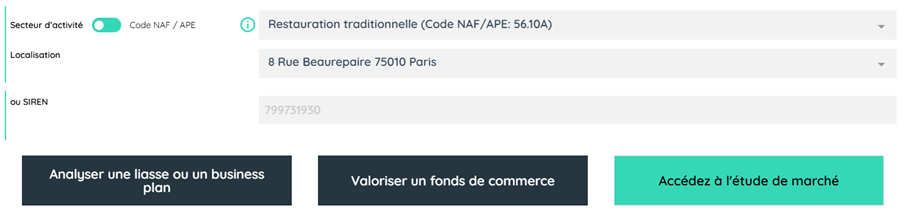
Source: atometrics.
Users simply select an industry (e.g., bakery, hairdressing) and a location, and Atometrics delivers a detailed report. This includes financial insights on competitors, transaction prices for nearby properties or businesses, valuation tools for businesses or shares, competitor mapping, and local demographic and economic data. Additionally, qualitative market insights are provided. The platform also features customizable email alerts to notify users of critical events, such as new tenders or competitors.
Report on a company.
Source: atometrics.
The platform allows users to either work with specific datasets (e.g., Excel exports, map visuals) or generate complete reports in PDF or PPT format.
Supporting small businesses at every stage
atometrics empowers small businesses through their stakeholders — accountants, banks, brokers, consultants — to access key information at the different stages of the business life cycle:
- Creation: assess market feasibility, validate business plans, and identify the best locations for new businesses.
- Development: monitor trends, spot opportunities, and manage risks. For example, our platform can alert managers to new competitors or relevant public tenders in real time.
- Difficulty phases: respond quickly to economic shifts with up-to-date market intelligence, ensuring resilience during challenging times.
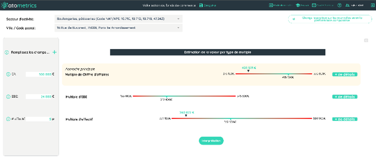
- Transmission and acquisition: conduct reliable valuations of businesses, assets, or securities based on accurate market multiples.
A concrete example: how atometrics enhances banking efficiency and risk assessment
Banks leveraging atometrics gain a significant advantage by accessing a uniform and structured source of information. When client managers and risk analysts evaluate a funding request or a business plan, they need to determine whether the entrepreneur is likely to achieve their revenue targets. This requires reliable market data: have similar projects succeeded or failed? Does the targeted catchment area show strong potential?
Atometrics simplifies this process by providing objective, data-driven insights that streamline the assessment of funding requests and accelerate the time to market of loan drawdowns. Instead of spending hours collecting and interpreting scattered information, bank advisors can access clear, actionable insights in real time.
Furthermore, the shared use of atometrics across commercial and risk departments fosters a common source of information among them, hence improving communication and collaboration between teams.
Conclusion
In today’s data-driven world, success belongs to those who can transform information into action. atometrics equips small business stakeholders with the tools and insights they need to unlock opportunities, navigate challenges, and drive sustainable growth—at every stage of the journey.
Why should I be interested in this post?
In today’s era of open finance and open data, financial professionals need cutting-edge tools to better serve their clients. This article reveals how atometrics, an innovative French fintech, is transforming the way banks, brokers, accountants, and business advisors support companies through data analytics. Whether you’re an ESSEC student preparing for a career in finance, a banker looking to streamline credit processes, or a consultant aiming to provide better market insights, you’ll want to know how the latest data-driven tools are reshaping financial decision-making and improving client service.
Related posts on the SimTrade blog
▶ Nithisha CHALLA Job description – Financial analysts
▶ Louis DETALLE The importance of data in finance
▶ Nithisha CHALLA Market Consensus Based on Financial Analysts’ Forecasts
Useful resources
About the authors
The article was written in January 2025 by Yann FONTAINE (head of Marketing of atometrics) and Sylvain GILIBERT (co-founder of atometrics).