Implied Volatility Surface: Smiles, Smirks and Term Structure

Saral BINDAL

In this article, Saral BINDAL (Indian Institute of Technology Kharagpur, Metallurgical and Materials Engineering, 2024-2028 & Research assistant at ESSEC Business School) explains the implied volatility surface: its characteristic shapes, static arbitrage constraints, and application using S&P 500 index options data.

Introduction

In financial markets characterized by uncertainty, volatility is a crucial factor in the valuation of derivative securities. For options traders, an option price is essentially volatility. Although options are traded at monetary prices, professionals routinely quote and compare them in terms of implied volatility (%), making volatility the common language of options markets. Moreover, in a reverse way, implied volatility occupies a central role as a forward-looking indicator that reflects the market’s expectations of future price fluctuations embedded in option prices.

Under the Black-Scholes-Merton (BSM) model, volatility is assumed to be constant and independent of option characteristics like the strike price (K) and the time to maturity (T). Empirical evidence, however, reveals that implied volatility varies across option contracts and especially depends on both parameters K and T of the option.

Implied volatility curves: the strike dimension

Volatility curves represent a cross-sectional view of the implied volatility surface (IVS), depicting the relationship between implied volatility and strike price for a fixed maturity. They are constructed by plotting implied volatility as a function of strike while holding time-to-maturity constant.

The volatility curves are commonly observed in two distinct shapes, most notably the volatility smile and the volatility smirk. A detailed discussion of the empirical relationship between implied volatility and option moneyness, the associated stylized facts, and their economic interpretation can be found in the article Volatility curves: smiles and smirks.

Figure 1 below illustrates the implied volatility smile (1a) and smirk (1b).

Figure 1a and 1b. Implied Volatility Smile and Smirk
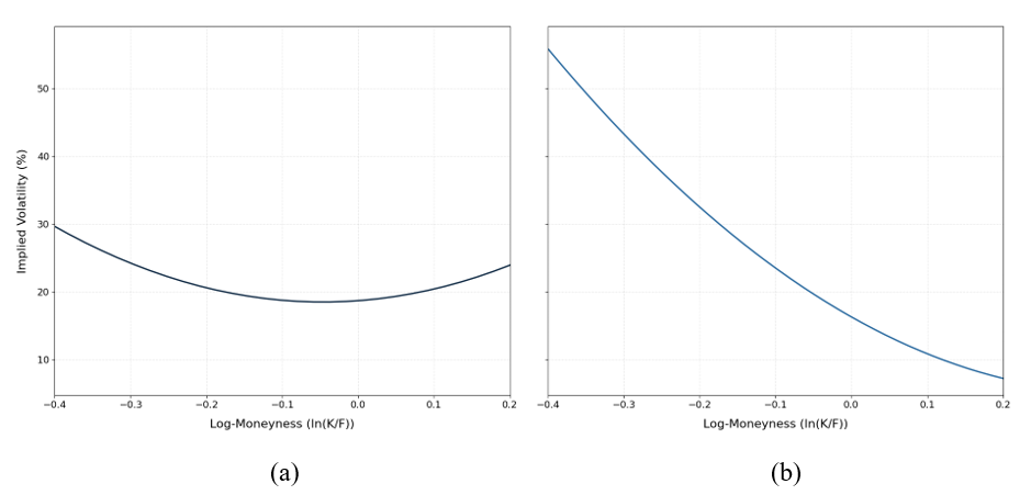
 Implied Volatility Curves (smile and smirk)
Source: computation by the author (with python).

Term structure of implied volatility: the maturity dimension

While volatility curves describe the strike dependence of implied volatility, the maturity dimension captures how implied volatility varies across expiration dates for a given strike. This relationship is commonly referred to as the term structure of implied volatility.

Using daily implied volatility data for S&P 100 index options (December 1983 to September 1987), Stein (1989) documented that volatility shocks are transmitted across maturities more strongly than predicted by standard rational expectations theory. Under this standard theoretical framework, because implied volatility is strongly mean-reverting, a near-term shock should naturally decay over time, causing long-dated implied volatilities to change by only a fractional amount. However, following an increase in short-dated implied volatility, long-dated implied volatilities tend to rise by a disproportionately large amount, indicating that changes in near-term uncertainty heavily influence market expectations over a broad range of maturities.

Using data for options on the S&P 500, FTSE 100, DAX 30, CAC 40, and Nikkei 225 stock indexes spanning the period May 9, 1994 to October 12, 2001, Mixon (2007) suggested mean reversion as a key characteristic of the implied volatility term structure. While short-dated implied volatilities exhibit substantial sensitivity to changes in market conditions, long-dated implied volatilities remain comparatively stable, reflecting expectations of convergence toward a long-run volatility level. Consequently, the term structure is generally upward sloping (contango) during periods of low market uncertainty but may become inverted (backwardation) during episodes of market stress, when short-term volatility rises sharply.

Figure 2 illustrates an upward-sloping (2a) and a downward-sloping (2b) implied volatility term structure.

Figure 2a and 2b. Implied Volatility Term Structure
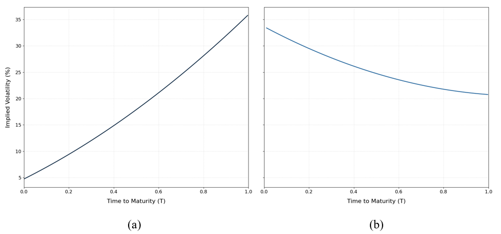
Implied Volatility Term Structure
Source: computation by the author (with python).

Christoffersen, Heston, and Jacobs (2009) demonstrate that the volatility term structure is not necessarily monotonic, arguing that capturing its true dynamics requires multifactor stochastic volatility frameworks. Evaluating European S&P 500 call options from 1990 through 2004, their empirical evidence reveals that implied volatility frequently displays significant curvature across maturities. This non-monotonic curvature is difficult to reconcile with traditional single-factor specifications like the benchmark Heston (1993) model, which restricts the term structure of implied volatility because it relies on only a single variance factor to model volatility over time.

Volatility Surface

The volatility surface provides a three-dimensional representation of implied volatility across strike prices and maturities. It is represented by the function σ(K,T), which assigns an implied volatility to each combination of strike price K and time to maturity T that reproduces the observed market option prices under the Black-Scholes-Merton (BSM) model.


Call option price formula under the BSM

Constructed from a cross-section of traded options, the volatility surface provides a comprehensive description of how the market prices uncertainty across both strike price (K) and maturity (T).

Arbitrage constraints

In practice, market option quotes are available only for a discrete set of strikes and maturities. Constructing a continuous volatility surface therefore requires interpolation and smoothing techniques. To ensure economic consistency, we must have σ(K,T) ≥ 0 for all strikes K and expirations T and the resulting surface must satisfy the static no-arbitrage conditions: namely the absence of butterfly arbitrage across strikes and calendar-spread arbitrage across maturities. (see, Breeden & Litzenberger, 1978; Gatheral, 2006)

The absence of butterfly arbitrage requires option prices to remain convex with respect to strike. Equivalently, the risk-neutral probability density implied by option prices must remain non-negative across all strikes, this condition can be expressed as:
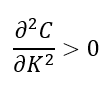

Conditon for the absence of butterfly arbitrage

A violation of this condition implies a negative risk-neutral probability density over some range of strikes and leads to arbitrage opportunities.

The absence of calendar-spread arbitrage states that with increase in maturity of an option, it should not result in a reduction of its value, since a longer-dated option provides all the rights of an otherwise identical shorter-dated option together with additional time for favourable price movements to occur. In volatility surface modelling, this condition is typically expressed in terms of the total implied variance
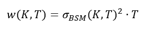

Total implied variance formula

where σBS(K,T) denotes the Black-Scholes-Merton implied volatility for strike K and maturity T. Total implied variance measures the total accumulated expected variance over the entire life of the option

For a fixed strike, total implied variance must be non-decreasing with maturity
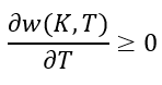

Conditon for the absence of calendar-spread arbitrage

A violation would imply that a longer-dated option embeds less cumulative uncertainty than a shorter-dated option at the same strike, resulting in an arbitrage opportunity.

Together, the butterfly-arbitrage and calendar-spread-arbitrage constraints ensure that the interpolated volatility surface produces arbitrage-free option prices and a valid risk-neutral distribution.

An Empirical Analysis of the S&P 500 Implied Volatility Surface

In this section, we discuss how an implied volatility surface can be estimated from the S&P 500 index observed market option prices using a parametric model to fit the data and how the parameters can be adjusted to represent different macro-economic stress conditions.

Data collection and filtration

To construct the implied volatility surface, we import the S&P 500 index option chain (set of call and put options across various strikes and maturities) directly from Yahoo! Finance. Because raw market data often contains stale quotes and asynchronous prices, we apply a robust set of filtering techniques to clean the dataset before model estimation.

First, we apply illiquidity filters, removing any option contracts with zero trading volume or zero open interest. Second, we filter the dataset to retain only Out-of-the-Money (OTM) options (OTM puts where K < S0, and OTM calls where K > S0). This is a standard practice, as implied volatility is theoretically independent of option type due to Put-Call Parity, focusing strictly on OTM contracts ensures we utilize the most liquid instruments (liquidity being measured by the bid-ask spread) to minimize pricing noise.

Third, we enforce intrinsic value and no-arbitrage boundary conditions. Any contracts with mispriced or economically impossible quotes are filtered out by verifying the upper and lower price bounds for the option contracts as given below
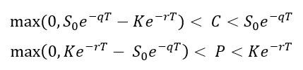

Call and Put option mid-price bounds

where:

  • K: strike price of the option
  • S0: spot price of the underlying asset
  • T: time to maturity
  • C: mid-price of a call option
  • P: mid-price of a put option
  • r: risk-free rate
  • q: continuous dividend yield

Finally, we check for vertical (strike) arbitrage to ensure the data adheres to fundamental shape restrictions. We sort the contracts by time-to-maturity and then by strike price in ascending order. We then verify shape monotonicity: for any given maturity, call prices must strictly decrease as the strike price increases, and put prices must strictly increase as the strike price increases. Applying these standard empirical filters ensures a clean, arbitrage-free dataset ready for surface estimation.

Methodology

To model and plot the implied volatility surface as shown below in Figure 1, we implement a parametric approach originally proposed by Dumas, Fleming, and Whaley (1998). This technique fits a deterministic volatility function (DVF) directly through the observed option market data. Under this framework, the implied volatility function is expressed as a second-order polynomial function across log-moneyness (M) and time-to-maturity (T):


DVF Formula

where:

  • α0 : Measures the baseline implied volatility level where both log-moneyness and time-to-maturity are equal to zero. Geometrically, this shifts the entire surface straight up or down uniformly
  • α1 : Measures the rate of change of volatility across different strikes. Geometrically, this rotates the surface along the moneyness axis, tilting the left wing (puts) up and the right wing (calls) down.
  • α2 : Measures the rate of change of the curvature across strikes, defining how sharply the volatility curve bends. Geometrically, this bends the surface into a U-shaped bowl or flattens it into a smooth plane.
  • α3 : Measures the rate of change of volatility across the horizon, establishing the slope of the term structure. Geometrically, this tilts the surface front-to-back, altering the premium difference between short-term and long-term contracts.
  • α4 : Measures the rate of change of the curvature in the volatility in the term structure across different maturities. Geometrically, this creates a non-linear bend along the time horizon axis.
  • α5 : Measures the co-dependency between moneyness and time-to-maturity, modelling how the skew changes as maturity extends. Geometrically, this causes the corners to bend upward or downward simultaneously.

In the polynomial function above, we utilize the log-forward moneyness (M), defined as:
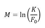

Log-forward moneyness formula

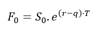
where F0 is the forward price of the underlying asset, calculated as:

Forward price formula

This is usually done in practice because it is F0, and not S0, that represents the expected stock price on the option’s maturity date in a risk-neutral world. Consequently, traders often define an “at-the-money” option as a contract where K = F0, rather than an option where K = S0.

To fit this model, we first apply a numerical root-finding algorithm to invert the Black-Scholes-Merton (BSM) pricing model against observed market prices (mid prices defined as the average of bid and ask prices) to extract the market implied volatilities. We restrict our sample to contracts with maturities under one year (T < 1.0) and a log-moneyness of |M| < 0.45. This filters out deep Out-of-the-Money (OTM) options, which typically suffer from low trading volumes and wide bid-ask spreads, as they are primarily held for structural tail-hedging by institutional investors.

Finally, we apply Ordinary Least Squares (OLS) regression to the filtered dataset to solve for the six α parameters simultaneously. Once estimated, these parameters can be used to generate the implied volatility curves, term structures, and 3D surfaces under various macroeconomic stress scenarios, as discussed below.

Empirical Results

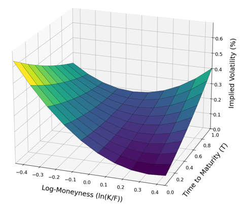
Figure 3 illustrates the estimated implied volatility surface of the S&P 500 index using options data collected on June 18, 2026. The market environment at the time of collection was defined by an index spot price (S0) of $7496.04, a risk-free interest rate (r) of 3.658%, and a continuous dividend yield (q) of 1.04%. Based on these inputs, the resulting empirical surface is presented below.

Figure 3. Implied Volatility Surface of the S&P 500 index options (June 18, 2026)
 Implied Volatility Surface of the S&P 500 options (June 18, 2026)
Source: computation by the author (with python).

From the surface, we can observe that amid ongoing US-Iran tensions in the Middle East, out-of-the-money (OTM) put options exhibit high implied volatility for short-term maturities. This reflects panic buying of downside protection due to fears of conflict escalation and immediate uncertainty in the market. Toward the far end of the maturity, however, the surface balances out with OTM call options. This indicates that while near-term sentiment is dominated by risk aversion, long-term market expectations are highly speculative, positioning for a potential recovery once the geopolitical uncertainty resolves. To isolate and observe these market dynamics more precisely, the individual implied volatility smiles (by strike) and term structures (by maturity) are plotted below.

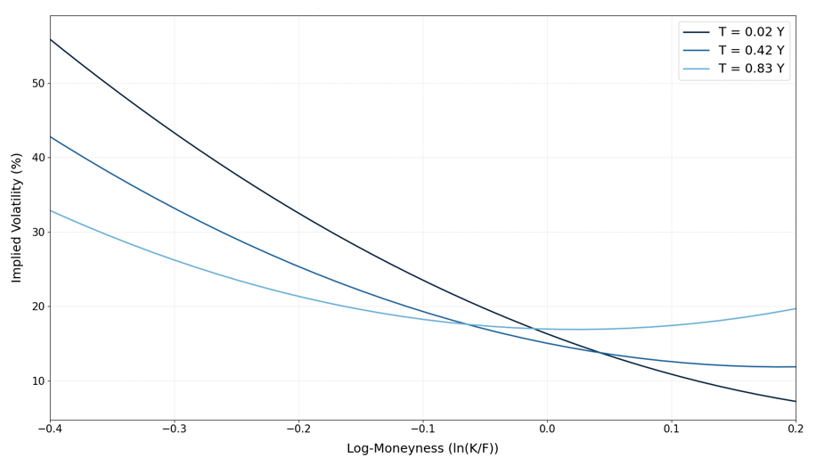
Figure 4 illustrates the implied volatility curves for three distinct maturities. As discussed above, we can clearly observe the steep downside skew flattening out and transitioning into a asymmetric smile as maturity increases.

Figure 4. Implied Volatility Curves of the S&P 500 options (June 18, 2026)
 Implied Volatility Curves of the S&P 500 options (June 18, 2026)
Source: computation by the author (with python).

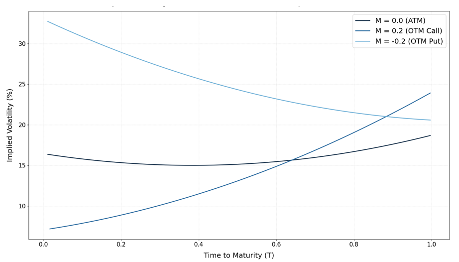
Figure 5 illustrates the implied volatility term structure (up to 1 year) for three different strike prices. For out-of-the-money (OTM) call options, we can observe that the term structure is upward-sloping, indicating a long-term uncertainty alongside expectations of an upward market movement. Conversely, the OTM put option term structure is inverted and reflecting high short-term panic and uncertainty. Over the time horizon, this near-term panic subsides, balancing out with the OTM call options in the long run.

Figure 5. Implied Volatility Term Structure of the S&P 500 index options (June 18, 2026)
Implied Volatility Term Structure of the S&P 500 index options (June 18, 2026)
Source: computation by the author (with python).

The at-the-money (ATM) option term structure exhibits a shallow, non-monotonic U-shape, characterized by elevated short-dated volatility, a flattened middle region, and higher long-term volatility. This reflects that, in the short-to-medium term, the curve demonstrates the classic mean-reversion, where the immediate geopolitical shock dissipates and flattens out over a 3-to-6-month horizon. Conversely, the upward drift at the longer end of the mature horizon reflects the structural term premium demanded by investors to account for broader, open-ended macroeconomic uncertainties, as discussed above in the stylized facts section.

Structural Shifts under Macroeconomic Stress: A Comparative Scenario Analysis

Figure 6 provides a compelling visual framework for observing how the implied volatility surface structurally shifts under different stress conditions. The surface on the left (a) represents the systemic crash caused by the COVID-19 pandemic (2020), while the surface on the right (b) illustrates the hypothetical impact on index options if the ongoing US-Iran conflict were to escalate significantly. These surfaces are constructed by adjusting the values of the six model parameters estimated in the preceding section; as such, they serve as illustrative examples of structural shifts rather than exact numerical forecasts.

Figures 6a and 6b. Implied Volatility Surface of the S&P 500 options under different stress environments
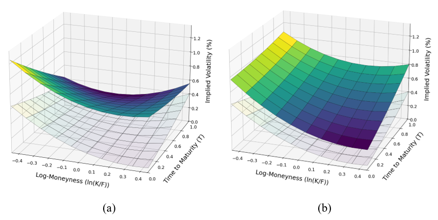
Implied Volatility Surface of the S&P 500 options under different stress environments
Source: computation by the author (with python).

Note: In both figures, the lightly shaded surface serves as the baseline, representing the actual market implied volatility surface as of June 18, 2026.

From Figure 6a, we can observe a massive surge in overall implied volatility across the board, driven by widespread panic buying of both out-of-the-money (OTM) puts and calls. This systemic shock resulted in a relatively flatter skew but severe inversion across the maturity spectrum, reflecting the acute, immediate fear of economic collapse as global lockdowns were implemented.

In contrast, Figure 6b models a scenario where the US-Iran conflict escalates into a full-scale regional crisis. Such an event would severely disrupt global oil supply chains, acting as a prolonged macroeconomic drag that hits S&P 500 corporate earnings over many months. Because this represents a lingering economic threat rather than an overnight liquidity freeze, the market’s response is highly asymmetric: demand is heavily concentrated in OTM puts for long-term downside protection and a steady increase in long-term implied volatility across the maturity.

While these stress scenarios represent extreme events, day-to-day movements follow structured patterns. Cont and Da Fonseca (2002) showed that daily dynamic deformations of the S&P 500 volatility surface are not chaotic. Instead, using principal component analysis, they demonstrated that surface movements are driven by just a few common statistical factors: parallel shifts, changes in the strike slope (skew), and twists in the maturity curvature.

You can download the Python code provided below, for the construction of the implied volatility curves, term structures and surfaces under different stress conditions as discussed above.

 the construction of the implied volatility curves, term structures and surfaces.

Alternatively, you can download the R code below with the same functionality as in the Python file.

Download the R code for the construction of the implied volatility curves, term structures and surfaces.

You can download the cleaned S&P 500 index options data for 18 June 2026, as used in the above Python and R codes to make the plots as discussed before.

Download the cleaned S&P 500 index options data

Volatility Surface Models

A volatility surface determines the risk-neutral distributions implied by option prices (see Option Implied Risk-Neutral Distribution), but it does not uniquely specify the underlying stochastic process governing asset-prices. As highlighted by Cont (2006), this introduces significant model uncertainty: different mathematical frameworks can calibrate perfectly to the exact same market volatility surface today, yet yield wildly divergent prices and hedges for exotic options because they imply different future surface dynamics. Consequently, a substantial body of research has focused on developing models capable of reproducing both the observed shape of the volatility surface and its evolution through time.

The principal modelling approaches include local volatility models, stochastic volatility models, parametric surface models and, more recently, rough volatility models.

Local Volatility Models

In the standard BSM formula, volatility is assumed constant, which however does not correspond to reality, as markets exhibit volatility smile and skews. Local volatility model, extends the BSM, by assuming that volatility is a function of stock price (St) and time (t), and the instantaneous local volatility is given by σt( St,t).

The Dupire (1994) formula that links the instantaneous local volatilities, to the implied volatility surface is given as follows:
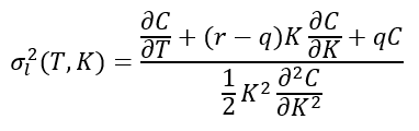

Local volatility formula

Stochastic Volatility Models

Stochastic volatility refers to the modelling of volatility using time-dependent stochastic processes, in contrast to the constant volatility assumption made in the standard BSM model. These models are better able to capture the observed features such as volatility clustering and mean reversion. One of the most widely used stochastic volatility models is the Heston (1993) model. The model describes the dynamics of the underlying asset price and its variance using a system of two coupled stochastic differential equations (SDEs), given by:
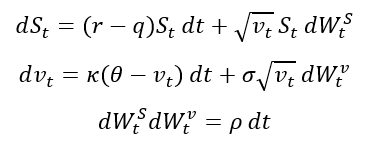

Stochastic volatility formula

Where:

  • St: is the asset price
  • vt: is the instantaneous variance
  • r: is the risk-free interest rate
  • q: is the continuous dividend yield
  • κ: is the speed of mean reversion
  • θ: is the long-run variance level
  • σ: is the volatility of variance (volatility-of-volatility)
  • ρ: is the correlation between shocks to the asset price and variance

Parametric Surface Models

Parametric volatility surface models are used to interpolate and extrapolate implied volatility across strikes and maturities, for sparse or illiquid strikes and ensure the resulting surface is free from static arbitrage (butterfly and calendar arbitrage).

Among the most widely used approaches is the SVI (Stochastic Volatility Inspired) parametrization, developed by Gatheral and Jacquier (2014), which is commonly applied to equity and index volatility surfaces. It models the total implied variance as a function of log-moneyness, providing a parsimonious representation of the volatility smile.

Other important parametric frameworks include the SABR model (Stochastic Alpha, Beta, Rho), which is widely used in interest rate and FX markets, and SSVI (Surface SVI), which extends the SVI framework to ensure arbitrage-free surface dynamics across maturities.

Rough Volatility Models

Rough volatility models represent one of the most important recent developments in volatility modelling. Gatheral, Jaisson, and Rosenbaum (2018) provided the empirical evidence that log-volatility behaves essentially as a fractional Brownian motion with Hurst exponent H of order 0.1, at any reasonable timescale.

The Hurst exponent (H) is a statistical parameter that characterises the roughness of a stochastic process: when H = 0.5, the process reduces to a standard Brownian motion with no memory, corresponding to a random walk. Whereas, values of H > 0.5 indicate persistent behaviour, while H < 0.5 imply anti-persistence, where increments tend to reverse direction more frequently, leading to rougher sample paths.

This observation, led to adoption of the fractional stochastic volatility (FSV) model of Comte and Renault (1998). The Rough FSV (RFSV) in contrast to FSV, is remarkably consistent with financial time series data. Compared to classical stochastic volatility models, it better captures the extremely rough nature of volatility paths and enables improved forecasting of realized volatility.

Why should I be interested in this post?

Implied volatility surfaces are among the most important tools in modern quantitative finance. They play a central role in the pricing and hedging of derivatives, particularly exotic options, and are widely used in risk management, stress testing, and scenario analysis. A good understanding of volatility surfaces is therefore essential for students, practitioners, and anyone seeking a career in derivatives, quantitative finance, trading, or risk management.

Related posts on the SimTrade blog

   ▶ Saral BINDAL Historical Volatility

   ▶ Saral BINDAL Implied Volatility and Option Prices

   ▶ Saral BINDAL Volatility curves: smiles and smirks

   ▶ Saral BINDAL Option Implied Risk-Neutral Distribution

Useful resources

Academic research on Option pricing

Black, F., & Scholes, M. (1973). The pricing of options and corporate liabilities. Journal of Political Economy, 81(3), 637-654.

Breeden, D. T., & Litzenberger, R. H. (1978). Prices of state-contingent claims implicit in option prices. Journal of Business, 51(4), 621-651.

Hull J.C. (2015) Options, Futures, and Other Derivatives, Eleventh Edition, Global Edition, Chapter 15 – The Black-Scholes-Merton model, 338-369.

Merton, R.C. (1973). Theory of rational option pricing. The Bell Journal of Economics and Management Science, 4(1), 141-183.

Academic Research on Stylized Facts on Option Volatility

Christoffersen, P., Heston, S., & Jacobs, K. (2009). The shape and term structure of the index option smirk: Why multifactor stochastic volatility models work so well. Management Science, 55(12), 1914-1932.

Heston, S. L. (1993). A closed-form solution for options with stochastic volatility with applications to bond and currency options. The Review of Financial Studies, 6(2), 327-343.

Mixon, S. (2007). The implied volatility term structure of stock index options. Journal of Empirical Finance, 14(3), 333-354.

Stein, J. C. (1989). Overreactions in the options market. Journal of Finance, 44(4), 1011-1023.

Academic Research on Empirical Analysis of Implied Volatility Surfaces

Cont, R., & Da Fonseca, J. (2002). Dynamics of implied volatility surfaces. Quantitative Finance, 2(1), 45-60.

Gatheral, J. (2006). The Volatility Surface: A Practitioner’s Guide. John Wiley & Sons, Chapter 2 – Implied Volatility Surface, 25-42.

Hull J.C. (2015) Options, Futures, and Other Derivatives, Eleventh Edition, Global Edition, Chapter 20 – Volatility smiles and volatility surfaces, 451-467.

Dumas, B., Fleming, J., and Whaley, R.E. (1998). Implied volatility functions: Empirical tests. The Journal of Finance, 53(6), 2059-2106.

Academic Research on Implied Volatility Surface Models

Comte, F., & Renault, E. (1998). Long memory in continuous-time stochastic volatility models. Mathematical Finance, 8(4), 291-323.

Cont, R. (2006). Model uncertainty and its impact on the pricing of derivative instruments. Mathematical Finance, 16(3), 519-547.

Dupire, B. (1994). Pricing with a smile. Risk, 7(1), 18-20.

Gatheral, J., & Jacquier, A. (2014). Arbitrage-free SVI volatility surfaces. Quantitative Finance, 14(1), 59-71.

Gatheral, J., Jaisson, T., & Rosenbaum, M. (2018). Volatility is rough. Quantitative Finance, 18(6), 933-949.

Heston, S. L. (1993). A closed-form solution for options with stochastic volatility with applications to bond and currency options. Review of Financial Studies, 6(2), 327-343.

About the author

The article was written in June 2026 by Saral BINDAL (Indian Institute of Technology Kharagpur, Metallurgical and Materials Engineering, 2024-2028 & Research assistant at ESSEC Business School). His interests include tracking geopolitical developments and analysing their direct impact on macroeconomic factors such as inflation, trade balances, and currency volatility, with a focus on using data to quantify these global economic ripple effects.

Discover all posts written by Saral BINDAL.
CBOE Volatility Index

Saral BINDAL

In this article, Saral BINDAL (Indian Institute of Technology Kharagpur, Metallurgical and Materials Engineering, 2024-2028 & Research assistant at ESSEC Business School) explains the CBOE methodology for the construction of the volatility index or ‘VIX’.

Introduction

The Chicago Board Options Exchange (CBOE) Volatility Index, or VIX, is a real-time market index designed to measure the market’s expectation of 30-day forward-looking annualized volatility. It is option-based, calculated using the market prices of S&P 500 index options to gauge expected volatility.

History

In 1993, CBOE Global Markets introduced the CBOE Volatility Index (VIX Index). Originally designed by Robert E. Whaley (1993) to measure the market’s expectation of 30-day volatility, the index was calculated using an option-pricing model to derive the implied volatility of at-the-money S&P 100 index (OEX Index) options. The VIX Index quickly became the premier benchmark for U.S. stock market volatility and is widely referred to as the market’s “fear gauge”.

Ten years later in 2003, CBOE partnered with Goldman Sachs to completely overhaul the index. This update introduced a methodology independent of option-pricing models, adapting the seminal theoretical framework for model-free implied variance established by Britten-Jones and Neuberger (2000) alongside the practical replication insights of Demeterfi et al. (1999). This modern version of the VIX shifted its underlying base to the broader S&P 500 index. Rather than tracking a narrow selection of options, it estimates market expectations by aggregating a heavily weighted cross-section of SPX puts and calls across a wide range of strike prices.

Academic research confirms that this model-free aggregation method captures more information and provides a more efficient forecast of future realized volatility than individual Black-Scholes implied volatilities (Jiang & Tian, 2005).

Market Behavior

While VIX is often regarded as the market’s fear index, it might give one a false impression that it moves opposite to the S&P 500. Mathematically it has no directional bias, and only measures the magnitude of expected volatility. Instead, the real-world inverse relationship is driven by corporate capital structures and asymmetric investor behavior. As Black (1976) pointed out, when a stock price drops, a company’s financial leverage automatically increases, making the equity riskier and naturally driving up volatility.

Furthermore, market sell-offs trigger a sudden panic where investors rush to buy portfolio insurance (put options) all at once. Because the supply of this insurance is limited, options market makers must aggressively raise prices to protect themselves. Gârleanu et al. (2009) formalize this mechanism, demonstrating that because market makers cannot perfectly hedge their positions, concentrated investor demand directly drives option pricing and inflates implied volatility premiums. Since the VIX is calculated directly from these option prices, this demand-pressure mechanically forces the index to spike.

This same demand explains why the S&P 500 and the VIX occasionally rise together. During massive market rallies, investors experience FOMO (Fear of Missing Out) and rush to buy upside call options, or quickly buy puts to lock in their rapid gains. Just like during a market crash, this sudden increase in demand for options overwhelms market makers. To protect themselves, they hike option prices, which mechanically forces the VIX up even as the stock market climbs.

Option Selection Procedure

Selecting Eligible Expiration Dates

The VIX is designed to measure the market’s expectation of volatility over the next 30 calendar days. However, listed S&P 500 options rarely expire exactly 30 days from the calculation date. To address this, the methodology selects two option maturities: a near-term maturity of less than 30 days and a next-term maturity of more than 30 days remaining. Variance estimates are calculated for both maturities and subsequently interpolated to obtain a constant 30-day measure of expected volatility.

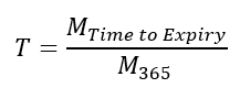
In the CBOE volatility index calculation methodology, time to expiration of a constituent option series, is calculated by dividing the number of minutes until expiration (MTime to Expiry) of the selected options (rounded down to the nearest minute) by the number of minutes in a year (M365).


VIX Time to Expiration Formula

Estimating the Forward Index Level

The next step is to estimate the forward index level of the S&P 500 using option markets prices. It represents the market’s expectation of the index value at expiration under the risk-neutral measure and serves as the reference point for selecting the relevant option contracts used in the calculation.

It is calculated using the principle of put-call parity, specifically by finding the unique strike price where the price difference between the call and the put option is at its absolute minimum.


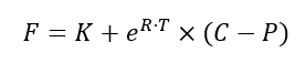
VIX Forward Price Formula

Where:

  • F: The forward index level
  • K: The smallest strike price at which the absolute difference between the call price and the put price is the smallest (|C – P| is minimized).
  • C: The market price (midpoint of the bid-ask spread) of the call option at the strike price Kmin.
  • P: The market price (midpoint of the bid-ask spread) of the put option at the strike price Kmin.
  • R: The risk-free interest rate (typically based on U.S. Treasury bills matching the option’s maturity).
  • T: The time to expiration (expressed as a fraction of a calendar year).

Determining K0

Once the forward index level has been estimated, we then identify K0, defined as the first strike price equal to or immediately below the forward index level (F). This strike acts as a reference point for the option selection process, separating the out-of-the-money put options from the out-of-the-money call options used in the calculation.

Selecting Out-of-the-Money Options

The VIX methodology uses a wide range of out-of-the-money (OTM) put and call options. OTM options are sensitive to changes in expected future volatility and provide information about the market’s expectations across a broad range of potential future outcomes. By incorporating both downside and upside option prices, the methodology captures the entire market-implied distribution of future index values rather than relying on a single option contract.

Variance Calculation

The Contribution of Individual Options Contracts

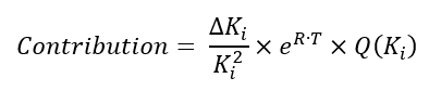
Each selected option contributes unique information about the market’s expectation of future variance. The weight of this contribution depends on three key factors: the option’s mid-price (Q(Ki)), the strike spacing (ΔKi) between neighbouring contracts, and the inverse square of its strike price (1/(Ki)2). This precise weighting scheme ensures that information from the entire out-of-the-money option chain is integrated into the final variance estimate.


VIX Option Contribution Formula

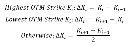
where for:


Strike Spacing Formula

The VIX Variance Formula

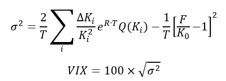
The option selection and weighting procedure described above is formally represented by the VIX variance formula. Rather than estimating volatility from a single option, the formula aggregates information from all selected option contracts to produce an estimate of expected future annualized variance.


VIX Variance Formula

Where:

  • σ2: Annualized variance
  • T: Time to expiration (in years)
  • F: Option-implied forward price
  • Ki: Strike price of the ith out-of-the-money option
  • K0: First strike equal to or otherwise immediately below the forward index level, F
  • ΔKi: Strike spacing for ith out-of-the-money option
  • Q(Ki): The mid-price of an option with strike Ki
  • R: Risk-free interest rate (with maturity equal to option expiration date)

Variance Estimates for Near-Term and Next-Term Options

Applying the variance formula to both the near-term and next-term options produces two separate estimates of expected future variance. The methodology calculates variance first because option portfolios can replicate future variance directly. As demonstrated by Demeterfi et al. (1999), a continuously weighted portfolio of out-of-the-money options across all strikes can replicate the payoff of a log contract, which is a theoretical derivative whose payout is tied to the logarithm of an asset’s price, making its returns purely dependent on variance rather than direction. Because a log contract captures total realized variance regardless of the asset’s price path, this foundational result allows expected future variance to be inferred directly and purely from observable option prices.

Constructing a Constant 30-Day Variance Measure

The variance estimates obtained from the near-term and next-term option maturities are linearly interpolated to obtain a constant 30-day estimate of annualized variance. Taking the square root converts variance into volatility, while multiplying by 100 expresses the result as a percentage. The resulting value is reported as the VIX index. The formula used in the interpolated CBOE volatility index calculation is as follows:


Interpolation Formula

Where:

  • MT1: The number of minutes until expiration of the near-term options
  • MT2: The number of minutes until expiration of the next-term options
  • MCM: The number of minutes in the given constant maturity term (30 days)
  • M365: The number of minutes in a 365-day year
  • Ti: MTi / M365
  • σi2: Variance of the i-th term

Interpretation of the VIX

For this section, we consider the S&P 500 index options data collected on June 18, 2026, with a spot price of $7,496.04 and a risk-free rate of 3.66%. Excel file with complete data and VIX calculations can be downloaded below.

Download the Excel file with complete dataset and VIX calculation

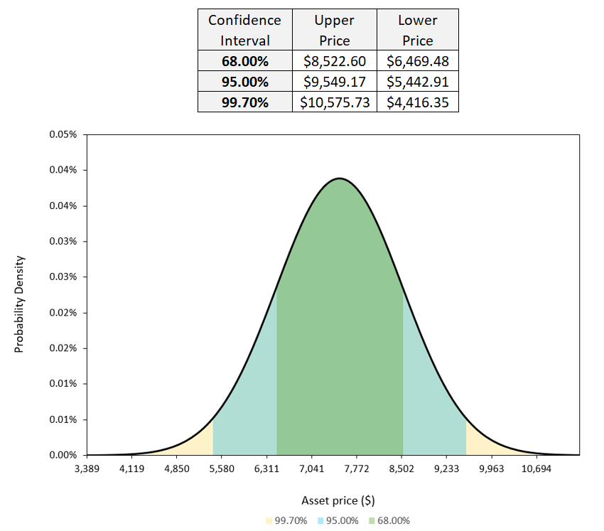
Our calculations yield a VIX value of 13.69, reflecting the market’s expectation of a ±13.69% movement over the next year. In Figure 1, we map this percentage onto a standard bell curve, where this expected movement in the S&P 500 index prices represent one standard deviation. This allows us to visualize the market’s expected range of price movements under the 68%, 95%, and 99.7% confidence intervals over the next one year.

Figure 1. Market Expected Price Over the Next 1 Year
Market Expected Price Over the Next 1 Year
Source: computation by the author.

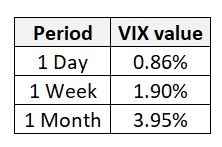
To calculate expected movements for shorter time frames, the VIX is scaled by dividing it by the square root of N, where N represents the number of periods in a year. For instance, N equals 12 to find a 1-month expected move, 52 for a 1-week move, and 252 trading days for a 1-day move.

Figure 2. Expected Movements for Shorter Time Frames
Expected Movements for Shorter Time Frames
Source: computation by the author.

You can download the Python code provided below, for VIX calculation using the modern CBOE methodology.

Download the Python code for VIX calculation.

Alternatively, you can download the R code below with the same functionality as in the Python file.

Download the R code for VIX calculation.

Why should I be interested in this post?

For anyone interested in finance or a career in trading, understanding how the VIX is constructed is crucial. As one of the most widely used measures of market uncertainty and expected volatility, it serves as an important tool for market analysis, risk assessment and numerous volatility-based trading strategies.

Related posts on the SimTrade blog

   ▶ Akshit GUPTA Options

   ▶ Jayati WALIA Black-Scholes-Merton Option Pricing Model

   ▶ Jayati WALIA Implied Volatility

   ▶ Saral BINDAL Implied Volatility and Option Prices

   ▶ Saral BINDAL Volatility curves: smiles and smirks

   ▶ Youssef LOURAOUI VIX index

Useful resources

Academic research

Black F. and M. Scholes (1973) The pricing of options and corporate liabilities. Journal of Political Economy, 81(3), 637–654.

Black, F. (1976), “Studies of Stock Price Volatility Changes”, Proceedings of the Business and Economics Section of the American Statistical Association, 177–181.

Britten-Jones, M. and A. Neuberger (2000) Option prices, implied price processes, and stochastic volatility. The Journal of Finance, 55(2), 839–866.

Demeterfi, K., Derman, E., Kamal, M., & Zou, J. (1999). A guide to volatility and variance swaps. The Journal of Derivatives, 6(4), 9-32.

Gârleanu, N., Pedersen, L. H., & Poteshman, A. M. (2009). Demand-based option pricing. The Review of Financial Studies, 22(11), 4259–4299.

Hull J.C. (2022) Options, Futures, and Other Derivatives, 11th Global Edition, Chapter 15 – The Black-Scholes-Merton model, 338–365.

Jiang, G. J. and Y. S. Tian (2005) The model-free implied volatility and its information content. The Review of Financial Studies, 18(4), 1305–1342.

Merton R.C. (1973) Theory of rational option pricing. The Bell Journal of Economics and Management Science, 4(1), 141–183.

Whaley, R. E. (1993). Derivatives on market volatility: Hedging tools long overdue. The Journal of Derivatives, 1(1), 71-84.

Business resources

Cboe Global Markets (February 26, 2026) Version 6.0 Cboe Volatility Index (VIX) Methodology.

Cboe Global Markets (February 26, 2026) Version 5.0 Cboe Volatility Index Mathematics Methodology.

About the author

The article was written in June 2026 by Saral BINDAL (Indian Institute of Technology Kharagpur, Metallurgical and Materials Engineering, 2024-2028 & Research assistant at ESSEC Business School). His interests include tracking geopolitical developments and analyzing their direct impact on macroeconomic factors such as inflation, trade balances, and currency volatility, with a focus on using data to quantify these global economic ripple effects.

Discover all posts written by Saral BINDAL.
Banca Monte dei Paschi di Siena — Learning Derivatives Sales from the Trading Floor

Marco SIMONETTI

In this article, Marco SIMONETTI (ESSEC Business School, MSc in Finance, 2025-2027) shares his experience as an Off-Cycle Sales & Trading Derivatives Intern at Banca Monte dei Paschi di Siena in Milan. The internship gave me direct exposure to how a corporate and investment banking desk transforms market information into practical hedging and trading solutions for corporate clients.

My role sits at the intersection of markets, corporate finance and client advisory. On one side, I follow macroeconomic and market developments in real time; on the other, I help translate those developments into concrete ideas for clients exposed to commodities, foreign exchange and interest rates.

About the company

Banca Monte dei Paschi di Siena (MPS) is one of the major Italian banking groups and is widely known as the world’s oldest bank still in operation, with origins in Siena in 1472. Today, the Group operates across retail banking, corporate banking, wealth management and capital markets activities.

My internship is based in Milan, within Sales & Trading Derivatives. The desk works with corporate clients that are exposed to fluctuations in commodity prices, exchange rates and interest rates. For example, an industrial company may need to hedge the cost of energy or raw materials, while an exporter may need to manage the risk that currencies move against its future revenues.

The value added by this type of desk is not simply to sell a financial product. It is to understand the client’s business model, identify the risk exposure, structure an appropriate solution and coordinate with traders to deliver an executable price. In other words, the role combines technical knowledge, market timing and commercial judgment.

Logo of the company.
Logo Bbanca Monte dei Paschi di Siena
Source: Banca Monte dei Paschi di Siena.

My experience as a Sales & Trading Derivatives Intern

My missions

Client coverage and needs identification: I supported the coverage of a portfolio of around 20 clients, helping identify hedging and trading needs across commodities, foreign exchange (FX) and interest rates. In practice, this meant understanding what each company buys, sells, imports, exports or finances, and how market volatility can affect its margins, cash flows and planning.

Market intelligence: I prepared real-time market reports and macro-driven trade ideas using Bloomberg. Bloomberg is a professional financial data platform used by banks, asset managers and corporates to monitor market prices, news, analytics and execution tools. My work involved following central-bank decisions, inflation data, interest-rate curves, energy markets and metals prices, then summarizing the implications for clients.

Product structuring: I worked on vanilla and semi-structured products such as forwards, swaps, options, collars and TARNs. A forward locks in a future price or exchange rate; a swap exchanges one stream of cash flows for another; an option gives protection or upside participation; a collar combines options to create a protection band; and a TARN (Target Redemption Note) is a structured product that terminates when a predefined target is reached.

Pricing and execution support: I worked day to day with traders to understand derivative pricing, bid-ask spreads and Greeks. The bid-ask spread is the difference between the price at which a dealer is willing to buy and the price at which it is willing to sell. The Greeks are risk measures used for options: for example, delta measures sensitivity to the underlying price, vega measures sensitivity to volatility and theta measures sensitivity to time decay.

Transaction process: I followed transactions from the client request to trade execution. This made me understand that the job requires both technical precision and process discipline: the client problem must be clearly identified, the structure must be suitable, the price must be executable and the documentation must be aligned with internal and regulatory requirements.

Commercial impact: From a core group of clients, the activity contributed approximately EUR 10k of daily revenues, primarily across oil & gas, energy and metals. This gave me a concrete view of how client relationships, market timing and product structuring can translate into measurable business results.

Required skills and knowledge

Hard skills: The internship requires knowledge of derivatives, fixed income, FX, commodities, option pricing, Bloomberg, macroeconomics, financial modeling and risk management. It also requires the ability to understand payoff profiles, compare hedging alternatives and interpret market data quickly.

Soft skills: The role also requires clear communication, attention to detail, speed under pressure and the ability to simplify complex market information. In derivatives sales, technical knowledge is useful only if it can be translated into a clear and relevant message for the client.

What I learned

The main lesson I learned is that derivatives sales is a bridge between markets and the real economy. A company does not hedge because a model says so; it hedges because volatility in oil, gas, metals, currencies or interest rates can directly affect its margins, debt service or investment plans.

I also learned that the quality of a trade idea depends on three elements: the market view, the client fit and the execution level. A correct macro view is not enough if the product is too complex for the client, too expensive to execute or misaligned with the company’s risk appetite.

Finally, the experience showed me the importance of discipline. Every price, spread, scenario and payoff profile must be checked carefully because derivatives can create both protection and risk. This is why sales and traders must work closely together before a transaction is executed.

Financial concepts related to my internship

I present below three financial concepts related to my internship experience:

Hedging with derivatives

Hedging means using financial instruments to reduce exposure to an unwanted risk. In my internship, typical risks include commodity price risk, FX risk and interest-rate risk. A commodity consumer may use swaps or options to stabilize future input costs; an exporter may use FX forwards to lock in an exchange rate; and a borrower may use interest-rate derivatives to reduce uncertainty around future financing costs.

Bid-ask spread and market making

The bid-ask spread is the difference between the price at which the bank can buy and the price at which it can sell a product. In derivatives, this spread compensates the bank for liquidity, hedging costs, market risk and operational complexity. Understanding the spread is important because it affects both the client’s execution level and the bank’s revenue.

Greeks and option risk management

The Greeks measure how the value of an option changes when market variables change. Delta measures sensitivity to the underlying price, gamma measures the change in delta, vega measures sensitivity to volatility, theta measures time decay and rho measures sensitivity to interest rates. These measures help traders hedge the risks created by client transactions and manage the desk’s exposure.

Why should I be interested in this post?

This post is relevant for ESSEC MiF students because it shows how financial theory becomes operational in a real banking environment. Courses on derivatives, portfolio management and financial markets provide the analytical foundation, but the internship shows how these tools are used under time pressure, with real clients and real market constraints.

For students interested in sales & trading, corporate banking or risk management, the role demonstrates that technical excellence and commercial understanding must go together. The best solutions are not necessarily the most complex ones, but the ones that are suitable, executable and useful for the client.

Related posts on the SimTrade blog

   ▶ All posts about Professional experiences

   ▶ Posts about derivatives and financial markets on the SimTrade blog

   ▶ Posts about trading and market making on the SimTrade blog

Useful resources

Banca Monte dei Paschi di Siena — Group website

Banca MPS — Commodity derivatives

Banca MPS — Foreign exchange derivatives

Banca MPS — Interest-rate derivatives

About the author

The article was written by Marco SIMONETTI (ESSEC Business School, MSc in Finance, 2025-2027), based on his experience as an Off-Cycle Sales & Trading Derivatives Intern at Banca Monte dei Paschi di Siena in Milan.

   ▶ Discover all articles by Marco SIMONETTI

Cristoforo Travel — From Zero to Exit: My Founder Story

Marco SIMONETTI

In this article, Marco SIMONETTI (ESSEC Business School, Master in Finance, 2025-2026) shares his founder experience building, scaling, and exiting Cristoforo Travel (2021-2025), a traveltech venture focused on B2B software and analytics for travel agencies and tour operators.

About the company

I founded Cristoforo Travel in early 2021 to help travel providers rebound after the pandemic with better technology and analytics. A traveltech company applies digital tools to the travel industry: for example booking engines, payment integrations, inventory management, pricing automation, customer data, and forecasting models. In our case, the objective was to help travel agencies and tour operators sell more efficiently, integrate fragmented systems, and use data to improve margins.

The company combined consulting with custom development to integrate booking and payment rails, automate inventory and pricing, and deliver lightweight forecasting tools. This hybrid model generated revenue quickly while compounding reusable IP. IP, or intellectual property, refers to proprietary assets that a company owns or controls; for Cristoforo Travel, this included connectors, software modules, analytics templates, and technical documentation that could be reused across clients. Reusing this IP reduced implementation time over successive engagements and made each new project easier to scale.

Our clients were mainly travel agencies and tour operators, ranging from independent agencies to larger B2B accounts. Among the most recognizable names, we worked with clients such as Alpitour and Evaneos. The value added was practical and measurable: we helped clients connect booking and payment systems, structure cross-selling flows, improve inventory visibility, and test pricing or demand assumptions with data instead of intuition. Cross-selling is now common across tourism: once a traveler buys a flight, hotel, or package, providers try to add insurance, transfers, activities, excursions, upgrades, or ancillary services. Our role was to make those add-on opportunities easier to manage and monetize for professional travel sellers.

The competitive landscape included traditional booking engines, travel CRM/ERP providers, destination-management software, and larger travel technology platforms used by agencies and tour operators. We competed less on brand size and more on flexibility, speed of integration, and the ability to combine product development with hands-on business consulting. Compared with large off-the-shelf platforms, our added value was the capacity to customize workflows for each client while gradually transforming repeated requests into reusable software modules.

Over time, I built a global partnership footprint – more than 90 partners across six continents – and secured enterprise-level agreements that pressure-tested reliability, security, and scale. Commercially, the business reached approximately €2 million in annual sales. As is typical in B2B travel services, gross margins were relatively low and varied by contract, usually between 5% and 20%, with an average of around 10% over five years. After operational costs and personnel expenses, the business generated approximately €30k-€40k per year of personal income for me, which I used to finance my studies abroad.

In June 2025, I sold my shares through a clean share sale. Due to confidentiality obligations, I cannot disclose the name of the acquiring company. However, I can say that it is listed on a Milan startup/SME stock market segment and operates with a business model very close to ours, which made the strategic fit natural.

Logo of the company.
Logo of Cristoforo Travel
Source: the company.

As founder and CEO, I led capital raising, product and delivery, sales and partnerships, and financial planning – owning the P&L, forecasting, and investor relations.

My experience as founder at Cristoforo Travel

My missions

Capital & financing: I raised €200k in seed funding from two angel investors to accelerate product and commercial rollout. I built a lean operating plan that linked hiring and product sprints to cash runway. Cash runway is the number of months a company can continue operating before running out of cash, based on its cash balance and monthly burn rate.

Product & delivery: I shipped integrations for booking and payments, pricing automation, and demand-forecasting tools. I balanced bespoke implementations with reusable modules: the first projects were more customized and lower-margin, but each engagement helped us identify features that could later become standardized modules.

Go-to-market: I created partnership playbooks, prospected and closed over 90 global partners, and established enterprise agreements with travel agencies and tour operators. I showcased our solutions at international trade fairs to generate pipeline, validate pain points directly with buyers, and compare our positioning against larger travel technology providers.

Data & strategy: I developed macro leading-indicator models for Southern Europe to guide market sequencing, inventory focus, and pricing experiments. These models helped prioritize which geographies, destinations, and product categories were more likely to convert depending on demand signals and seasonality.

Exit & integration: I negotiated a clean share sale in June 2025. A clean share sale means selling shares through a straightforward transaction with limited unresolved liabilities, clear ownership transfer, and clearly defined post-closing obligations. After the transaction, the technology and client logic were prepared for integration into the acquiring company, whose name I cannot disclose for confidentiality reasons. The acquirer is listed on a Milan startup/SME stock market segment and has a business model very similar to Cristoforo Travel.

Required skills and knowledge

Hard skills: financial modeling and runway management, pricing and unit economics, SaaS implementation and systems integration, data analysis for forecasting, and contract structuring, including SLAs, security, and compliance. SaaS means Software as a Service: software delivered online, usually through a subscription or recurring-fee model, instead of being installed and maintained locally by each client. SLA means Service Level Agreement: a contractual commitment that defines expected service quality, such as uptime, response times, support obligations, data protection, and remedies if service levels are not met.

Soft skills: enterprise sales storytelling, stakeholder management with investors, partners, and customers, cross-functional leadership, negotiation, and execution under uncertainty. In a small traveltech company, the founder often has to sell to clients, translate their operational problems into technical specifications, manage developers, and keep cash discipline at the same time.

What I learned

I learned that in traveltech, the best product ideas often come from concrete client problems. Our clients – travel agencies and tour operators, including accounts such as Alpitour and Evaneos – did not simply want software; they wanted fewer manual operations, better cross-selling, faster integrations, and more reliable data for pricing and inventory decisions. Competitors were often larger platforms or generic booking/CRM systems, but our advantage was speed, customization, and the ability to turn repeated client requests into reusable modules.

I also learned that consulting and development can fund product while accelerating learning. With around €2 million in annual sales, margins in B2B travel remained tight: contracts usually delivered 5%-20% gross margin, with an average around 10% over five years. This forced disciplined capital allocation. After costs and personnel, the company generated around €30k-€40k per year for me personally, enough to finance my studies abroad. That outcome taught me that a startup does not need to become a unicorn to create real value: it can also finance education, build professional credibility, and create strategic exit options.

Finally, selling at the edge of the roadmap validated security and compliance early, while clean interfaces and documentation made future M&A or platform integration smoother. The most important lesson was that sustainable growth depends on linking product decisions to client demand, cash discipline, and unit economics rather than chasing growth for its own sake.

Financial concepts related to my startup project

I present below three financial concepts related to my founder experience:

Seed financing, dilution & runway

Raising €200k from angel investors required balancing valuation and dilution with the operating runway necessary to reach commercial milestones. I built cash-flow forecasts, set hiring gates, and linked product sprints to liquidity checkpoints to avoid premature scaling. In practice, runway management meant asking: how many months can we finance development, sales, and support before the next cash inflow or funding milestone?

Unit economics & operating leverage

Our hybrid model began with lower margins from custom work but improved contribution as reusable modules, connectors, and templates reduced delivery time. Tracking gross margin by engagement type and CAC payback by partner cohort guided where to standardize and where to remain bespoke. Since B2B travel margins can be low, the key was to increase repeatability: each reusable connector or analytics template improved future unit economics.

Valuation, deal structure & integration

For my share sale in June 2025, I evaluated considerations beyond the headline price: representations and warranties, transition obligations, confidentiality, and the strategic value of integration into a listed company with a similar business model. Clean interfaces and documentation lowered integration risk and preserved the long-term value of the technology.

Why should I be interested in this post?

If you are an ESSEC MiF student curious about venture building or fintech-adjacent B2B business models, my story shows how financial discipline can combine with product-market execution to create real optionality. B2B means business-to-business: a company sells products or services to other companies rather than directly to consumers. In my case, Cristoforo Travel sold to travel agencies and tour operators, so success depended on enterprise trust, integrations, contract discipline, and measurable ROI for professional clients.

The broader advice is simple: start from a painful operational problem, sell early, measure margins contract by contract, document everything, and build reusable assets whenever a client request repeats. That combination can support profitable growth, finance personal and academic goals, and make a strategic exit more credible.

Related posts on the SimTrade blog

   ▶ All posts about Professional experiences

   ▶ All posts tagged Startups on the SimTrade blog

   ▶ Emanuele GHIDONI Reinventing Wellness: How il Puro Brings Personalization to Nutrition

   ▶ Alessandro MARRAS Venture Capital 101: A Quick Overview

   ▶ Quentin BONNEFOND Palantir: a potential and controversial rising decacorn

Useful resources

Italian Ministry of Enterprises and Made in Italy — Startup innovative

Registro Imprese — Start-up innovative

Alpitour — Company website

Evaneos — Company website

About the author

The article was written in June 2026 by Marco SIMONETTI (ESSEC Business School, Master in Finance, 2025-2026).

   ▶ Discover all articles by Marco SIMONETTI

Option Implied Risk-Neutral Distribution

Saral BINDAL

In this article, Saral BINDAL (Indian Institute of Technology Kharagpur, Metallurgical and Materials Engineering, 2024-2028 & Research assistant at ESSEC Business School) explains how option prices can be used to build an implied risk-neutral distribution.

Introduction

Derivative markets provide a rich source of information for market expectations. For example, a futures price is the market’s expectation of the future value of an asset. More interestingly, we can derive the moments of the statistical distribution of future asset values from the market prices of options, like the variance (second moment), the skewness (third moment) and the kurtosis (fourth moment). More generally, we can extract the ex-ante risk-neutral probability distribution of future asset prices at a given date from option market prices with the corresponding maturity date.

Physical vs Risk-Neutral Probability Measures

A real-world probability measure represents the statistical distribution of asset returns typically estimated using historical data. These measures incorporate risk premia, market frictions, and investor behaviour, and are primarily used for statistical inference and risk modelling.

In contrast, risk-neutral probability measure is a mathematical pricing measure used in no-arbitrage valuation of financial derivatives. Under this framework, asset prices are evaluated as discounted expected payoffs under an equivalent martingale measure. In this setting, the expected return of any risky asset is adjusted to the risk-free rate within the pricing measure, simplifying valuation by transforming uncertain future payoffs into present values computed via expectation (Hull, 2018; Shreve, 2004).

Historical vs Risk-Neutral Distributions

Historical Distributions are constructed from observed past returns under the physical measure (P-measure). They empirically capture the true statistical behaviour of asset prices, including fat tails, skewness, and volatility clustering driven by real market shocks and investor behaviour. These distributions exhibit higher variance and kurtosis, making them particularly valuable for stress testing, Value-at-Risk estimation, and portfolio risk management where realistic loss scenarios matter.

Risk-Neutral Distributions are derived from option market prices rather than historical data, under the implied measure by no-arbitrage pricing (Q-measure). They reflect market-implied expectations of future payoffs discounted at the risk-free rate resulting in smoother, less skewed densities. While highly effective for pricing derivatives and contingent claims, they tend to underestimate tail risk and do not directly represent the actual probabilities investors assign to future market outcomes.

Risk-neutral distribution: the Black–Scholes–Merton framework

Having distinguished between the physical and risk-neutral probability measures, it is useful to examine the risk-neutral distribution implied by the Black–Scholes–Merton (BSM) model, which is a standard model in quantitative finance. The BSM framework assumes that the underlying asset follows a geometric Brownian motion and provides a simple illustration of how the transition from the physical measure to the risk-neutral measure alters the distribution of future asset prices.

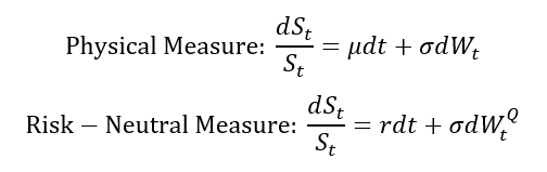
Under the BSM, the standard assumption is that the underlying asset follows a geometric Brownian motion given by the following expressions:


SDE for the geometric Brownian motion (GBM)

where:

  • St = asset price at time t t
  • μ = drift (growth rate of the asset price)
  • r = risk-free rate
  • σ = volatility (standard deviation)
  • dWt/dWtQ = infinitesimal increment of wiener process (N(0,dt)) under respective measures

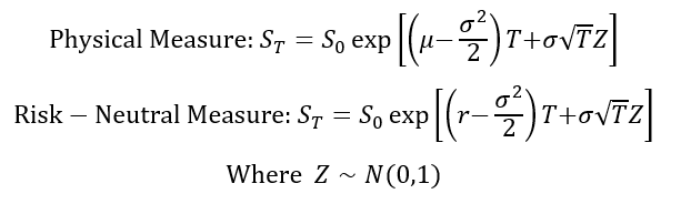
Solving these stochastic differential equations over the interval [0, T] yields the terminal asset price:


Terminal asset price formulas

Taking logarithms shows that the terminal log-price is normally distributed:


Distributions under the BSM framework

Thus, under the Black–Scholes–Merton framework, the risk-neutral distribution of the terminal asset price is lognormal (as the physical distribution). Relative to the corresponding physical distribution, the volatility remains unchanged, while the drift parameter μ is replaced by the risk-free rate r. This is an important result as the risk-free rate r is known and easily observable while the drift parameter μ has to be estimated and is not directly observable.

Butterfly spread

To extract a continuous risk-neutral probability distribution from the market, we must first understand how to isolate the market’s view on a specific future asset price. The primary tool for this is a classic option trading strategy: the butterfly spread.

A butterfly spread is an options trading strategy designed to achieve limited profit with strictly bounded risk, typically in market environments where relatively small price movements are anticipated. The strategy may be implemented using either call or put options and can be established in either a long or short configuration. For example, a long call butterfly is constructed by purchasing one call option at a lower strike price, selling two call options at an intermediate strike price, and purchasing one call option at a higher strike price. Depending on the relative spacing between the strike prices, a butterfly spread may be either symmetric or asymmetric.

Cost of a Symmetric Butterfly Spread

To understand how option market prices encode the market’s expectations regarding the future distribution of the underlying asset price, we consider a symmetric butterfly. A symmetric butterfly spread is constructed using three European call options with a common maturity T and distinct strike prices. The strategy involves purchasing one call option with strike K – ΔK at a premium of C(K-ΔK,T), selling two call options with strike K at a premium of C(K,T) each, and purchasing one call option with strike K + ΔK at a premium of C(K+ΔK,T).

The price of the resulting butterfly spread is therefore given by


Butterfly spread cost

The net cost of the butterfly spread is obtained by summing the premia paid for the two long call positions and subtracting the premiums received from the two short call positions.

Payoff of a Symmetric Butterfly Spread

The payoff of a symmetric butterfly spread is centred around the strike (K) and can be expressed as


Butterfly spread payoff

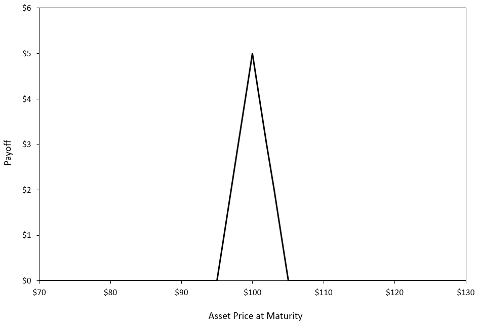
Figure 1 illustrates the payoff profile of a symmetric butterfly spread centred at the strike K = 100 with strike spacing ΔK = 5. The payoff reaches its maximum when the terminal asset price ST equals the strike K and declines to zero as ST moves beyond the adjacent strikes K – ΔK and K + ΔK.

Figure 1. Symmetric Butterfly Spread Payoff at Maturity
Symmetric Butterfly Spread Payoff  at Maturity
Source: computation by the author.

As a result, the butterfly spread effectively isolates a narrow range of terminal asset prices, making it a useful instrument for extracting information about the market-implied probability distribution of the underlying asset price at maturity.

Stacked Butterfly Spreads

A stack of butterfly spreads refers to a collection of butterfly spreads constructed across a range of strike prices, such that the central strike of each butterfly is equally spaced from the next. The spacing between successive central strikes is equal to the strike spacing ΔK used in the construction of each individual butterfly spread, as discussed above.

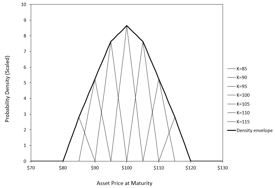
Figure 2 illustrates that a collection of butterfly spreads across strikes at a fixed maturity converges to the market-implied probability density of the underlying asset. Each butterfly corresponds to a discrete approximation of the second derivative of option prices with respect to strike, and aggregating these across strikes recovers the risk-neutral density.

We construct seven butterfly spreads centered at strikes K = 85 to K = 115 in increments of 5, with strike spacing ΔK = 5. The weights are specified using a Gaussian distribution with mean μ = 100 and standard deviation σ = 10, reflecting an assumed market belief about the concentration of terminal prices. The payoff profile is scaled by a factor of 200 to improve visual readability, and it is normalized by ΔK2 to remain consistent with the second-order finite-difference interpretation of butterfly spreads as detailed below.

Figure 2. Approximating the Risk-Neutral Density Using Butterfly Spreads
Approximating the Risk-Neutral Density Using Butterfly Spreads
Source: computation by the author.

As the strike spacing ΔK is reduced, additional butterfly spreads can be constructed between existing butterfly spreads. Consequently, the stacked payoff profile becomes increasingly smooth and, in the limit, approaches a continuous representation of the implied probability distribution.

To better understand this limiting behaviour, it is useful to examine the properties of an individual butterfly spread. As the strike spacing ΔK decreases, the payoff of the butterfly spread becomes increasingly concentrated around its central strike. In the limit as ΔK → 0, the butterfly spread approaches an infinitesimally narrow peak centred at K.

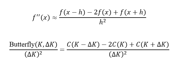
Consequently, the value of the butterfly spread decreases as its payoff becomes increasingly concentrated around its central strike. To obtain a meaningful limiting quantity, the butterfly value must therefore be normalized by (ΔK)2. This normalization is motivated by a well-known result from calculus, central finite-difference approximation of the second derivative.


Normalized Butterfly spread cost

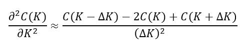
Comparing the two expressions above, reveals that the normalized butterfly value is precisely the finite-difference approximation of the second derivative of the call pricing function with respect to strike.


Second derivative of the call pricing function with respect to strike.

This observation forms the foundation of the Breeden-Litzenberger (1978) result, which establishes that the second derivative of the call pricing function with respect to strike is directly related to the market-implied risk-neutral probability density embedded in option prices, as demonstrated in the derivation below.

You can download the Excel file provided below to generate and visualize the payoff profiles of the butterfly spread and stacked butterfly spread at maturity, as discussed above.

Download the Excel file.

Option implied risk-neutral distribution

This section develops the analytical derivation of the risk-neutral distribution using the seminal Breeden-Litzenberger (1978) result. By exploiting the cross-sectional structure of option prices across strikes, we recover the market-implied risk-neutral density embedded in option market prices.

Analytical derivation

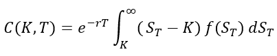
Under the risk-neutral measure, the value of a European call option is given by the present value of its expected payoff at maturity. For a strike price K, continuously compounded risk-free rate r, and time to maturity T, the call pricing function C(K,T) can be expressed as


Call option risk-neutral value.

To obtain a continuous representation of the call price, the expected payoff can be expressed as an integral over the probability density function of the terminal asset price, f(ST).


Call option risk-neutral value PDF.

Note: The integral starts at K because the payoff is zero when St≤K.

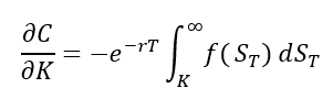
Taking the first derivative with respect to K, we get


Call option risk-neutral PDF first derivative

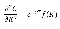
To obtain the risk-neutral probability density function, as shown by Breeden and Litzenberger (1978), we take an additional derivative with respect to the strike


Second derivative of call price with respect to strike.

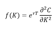
Rearranging the above formula, we get the risk-neutral distribution


Rearranged Second derivative of call price with respect to strike.

Applying the second-order central difference approximation heuristically developed in the previous section using butterfly spreads, we obtain the following expression:


Implied risk-neutral distribution formula.

This expression shows that the risk-neutral probability density can be recovered directly from the second derivative of the call pricing function with respect to strike. In practice, however, option prices are observed only at a finite set of discrete strike prices, requiring numerical methods to approximate the derivatives and extract the implied risk-neutral distribution.

Numerical methods for extracting the risk-neutral distribution

Methods for extracting the risk-neutral distribution can be broadly classified into non-parametric (data-driven with minimal distributional assumptions), semi-parametric (partial structural assumptions, typically imposed on intermediate quantities such as implied volatility), and parametric or structural (explicit assumptions on the distribution or asset price dynamics) approaches. These methodologies differ in the degree of modelling assumptions imposed on the option pricing function and the terminal asset price distribution, leading to different trade-offs between flexibility, numerical stability, and economic interpretability.

Non-parametric methods

Non-parametric methods aim to recover the risk-neutral distribution directly from observed option prices without imposing any specific parametric structure on either the terminal asset price distribution or the stochastic process governing the evolution of the underlying asset price. Consequently, these methods are highly flexible, but they tend to be sensitive to market microstructure noise, sparse strike coverage, and interpolation error in option quotes.

Risk-neutral histograms: the most direct implementation of the Breeden–Litzenberger result constructs a discrete approximation of the implied risk-neutral density using finite differences across traded strikes (Breeden and Litzenberger, 1978; Neuhaus, 1995). Adjacent butterfly spreads may therefore be interpreted as local estimates of state-contingent probabilities.

Because option contracts are quoted only at discrete strike intervals, the recovered distribution resembles a histogram rather than a smooth continuous density, making the approach highly sensitive to strike spacing and pricing noise.

Kernel regression methods: to mitigate the instability of histogram-based estimates, subsequent research introduced non-parametric smoothing techniques that estimate a continuous option pricing function directly from observed market prices. A prominent example is the kernel regression framework of Aït-Sahalia and Lo (1998).

By reducing the influence of local pricing noise, kernel-based methods generally produce smoother and more stable estimates of the implied risk-neutral density.

Spline-based methods: another widely used class of non-parametric methods employs spline interpolation techniques to construct smooth and arbitrage-consistent call pricing functions across strikes (Bates, 1991). Once a sufficiently smooth pricing function has been obtained, the implied risk-neutral density can be recovered through numerical differentiation.

Spline-based approaches offer substantial flexibility but remain sensitive to data quality and sparse observations in the tails of the distribution.

Semi-parametric approaches

Semi-parametric approaches occupy a middle ground between purely data-driven and fully parametric methodologies. Rather than modelling the risk-neutral density directly, these methods impose structure on intermediate quantities, most commonly the implied volatility smile.

Implied volatility smile methods: in practice, many market participants smooth the implied volatility smile rather than the option prices directly. Observed option prices are first converted into implied volatilities, after which a smooth volatility smile is fitted across strikes using parametric specifications or spline-based interpolation techniques (Shimko, 1993).

The smoothed volatility smile is subsequently mapped back into option prices, allowing the implied risk-neutral density to be recovered through numerical differentiation. These methods generally exhibit greater numerical stability, although tail estimation remains sensitive to extrapolation assumptions in illiquid regions of the smile.

Parametric and structural approaches

Parametric and structural methodologies recover the implied risk-neutral distribution by imposing explicit assumptions on either the terminal distribution of asset prices or the stochastic process governing their evolution.

Parametric density models: a prominent class of methods assumes that the terminal risk-neutral distribution follows a particular parametric specification. One widely used approach models the distribution as a mixture of lognormal densities calibrated to observed option prices (Bahra, 1997; Melick and Thomas, 1997).

Parametric methods are computationally efficient and often yield economically interpretable measures of skewness, kurtosis, and tail risk. Their flexibility, however, is inherently constrained by the assumed functional form.

Dynamic option pricing models: rather than specifying the terminal distribution directly, structural approaches derive the implied density from an assumed stochastic process governing the evolution of the underlying asset price. Examples include stochastic volatility and jump-diffusion frameworks calibrated to observed option prices (Bates, 1995; Malz, 1995).

Within these models, the risk-neutral density emerges endogenously from the dynamics of the underlying asset under the risk-neutral measure. While theoretically appealing, such models are computationally intensive and sensitive to model misspecification.

Application

Implementing the Breeden and Litzenberger (1978) result in practice requires a continuum of European option prices written on the same underlying asset, all sharing a common maturity and spanning a continuous range of strike prices from zero to infinity. Under such idealized conditions, the risk-neutral density can be recovered directly from the cross-section of option prices (at a given maturity date).

In practice, however, listed option markets provide only a sparse and discrete grid of strike prices, typically concentrated around the at-the-money (ATM) region. The absence of a complete continuum of option strikes, particularly in the deep in-the-money and far out-of-the-money regions, necessitates the use of interpolation across observed strikes and extrapolation into the tails in order to recover a smooth and arbitrage-free implied risk-neutral distribution.

Required data

Constructing a risk-neutral distribution requires option chain data (a set of calls and/or puts) for a single maturity, along with the underlying asset price, the prevailing risk-free rate, dividend assumptions, at the exact observation time of the market data.

Such data can be obtained from both free and commercial data providers. One of the most accessible sources is Yahoo! Finance; however, freely available option data is often subject to inconsistencies such as wide bid–ask spreads, stale quotes, and incomplete cross-sectional coverage of strikes, all of which can materially distort empirical estimation of the risk-neutral distribution (RND).

For our application, we employ simulated option data to illustrate the derivation of the implied risk-neutral distribution from an option chain within a controlled and internally consistent setting. This ensures that the resulting distribution remains aligned with the theoretical framework developed above.

Extraction of the implied risk-neutral density

From the collected option chain data, we first apply a series of standard filtering procedures designed to remove illiquid and economically inconsistent observations. In empirical applications, this typically includes liquidity screens, moneyness and maturity filters, implied-volatility sanity checks, and no-arbitrage constraints to mitigate errors arising from stale quotes, asynchronous observations, and market microstructure noise. Since the dataset employed here is simulated and internally consistent by construction, these preprocessing steps can be largely omitted.

Figure 3 below presents the implied volatility smile obtained from the simulated European call option chain after numerical inversion of the Black–Scholes–Merton pricing model. The smile is interpolated using a natural cubic spline over a dense strike grid spanning the filtered strike range of 4,000 to 6,000, under the assumptions of an underlying spot price of $5,300, a continuously compounded risk-free interest rate of 5.2%, and a remaining time-to-maturity of 30 days. The resulting smooth volatility curve serves as the key intermediate input for constructing a continuous and differentiable call pricing function required for subsequent risk-neutral density extraction.

Figure 3. Implied Volatility Smile
Implied Volatility Smile
Source: computation by the author (with python)

The interpolated implied volatility smile is subsequently utilized to reprice European call options across a finely discretized strike grid, thereby constructing a smooth numerical approximation of the cross-sectional call price surface. The option implied risk neutral density is then recovered by applying the Breeden Litzenberger operator, corresponding to the second partial derivative of discounted call prices with respect to strike, to the smoothed pricing function. Figure 4 illustrates the resulting risk neutral density extracted from the simulated European call option chain under an underlying spot level of $5,300, a continuously compounded risk-free interest rate of 5.2%, and a remaining time to maturity of 30 days.

Figure 4. Implied Risk-Neutral Distribution
Implied Risk-Neutral Distribution
Source: computation by the author (with python)

You can download the Python code provided below for generating simulated call option chain data and the option-implied risk-neutral distribution, as discussed above.

Download the Python code.

Alternatively, you can download the R code below with the same functionality as in the Python file.

 Download the R code.

Empirical issues

A primary limitation in empirical recovery of the risk-neutral distribution is the discrete nature of listed option strikes. The Breeden–Litzenberger framework assumes a continuum over strike space, whereas traded options are observed only on a sparse and uneven grid concentrated around the at-the-money region.

A second limitation arises from the unobservability of the distribution tails. Deep in-the-money and far out-of-the-money options are often illiquid or not quoted, implying that tail behaviour of the risk-neutral density must be inferred through extrapolation rather than direct market observation.

A separate issue is asynchronous option quotes. Since option prices across strikes are not necessarily recorded simultaneously, the resulting cross-section may embed timing mismatches, introducing bias in the reconstructed pricing function. This is typically addressed using end-of-day settlement data or synchronized snapshots.

In addition, different levels of market liquidity (due to different levels of bid ask spreads for example) across strikes introduces noise and heterogeneity in observed quotes. Illiquid contracts may exhibit stale or unreliable prices, which can distort the implied volatility surface even after basic filtering.

Finally, the reconstruction procedure does not explicitly impose no-arbitrage conditions or global smoothness constraints across strikes. As a result, when option prices are interpolated to form a continuous surface, the fitted call price function may exhibit local violations of convexity in strike space (e.g., small regions where butterfly spreads imply negative prices or non-monotonic curvature). Such violations are problematic because they imply the possibility of arbitrage and can lead to risk-neutral probability estimates that are not economically consistent.

Despite these limitations, the framework remains a useful reduced-form tool for extracting risk-neutral densities, provided appropriate smoothing and arbitrage constraints are imposed.

Real-life applications

Central Bank Monetary Policy Monitoring

Bahra (1997) and Kim (2009) suggest that policymakers extract ex-ante risk-neutral distributions (RNDs) from interest rate, equity, and currency options to assess market-implied expectations and uncertainty around policy decisions. Unlike futures prices, which only reflect the conditional mean, RNDs incorporate higher-order information such as skewness and kurtosis, allowing for a more complete assessment of perceived tail risks and macro-financial stress. For example, during the February 2007 equity sell-off, the European Central Bank (ECB, 2007) used option-implied probability distributions (“fan charts”) to assess whether the move reflected extreme tail risk and to track the evolution of market expectations after stabilization.

Value-at-Risk (VaR) Forecasting

Risk management units in investment banks use quantiles derived from implied RNDs to forecast extreme portfolio losses in a forward-looking manner. Compared to traditional historical simulation methods, RND-based approaches incorporate market-implied expectations and have been shown to provide improved performance relative to standard volatility-based models such as GARCH(1,1) (Chang, Chang, Huang, & Hsieh, 2011).

Systemic Risk and Stress Testing Indicator

Macroprudential regulators transform option-implied volatility surfaces into arbitrage-consistent risk-neutral distributions to quantify system-wide financial vulnerabilities. By aggregating tail-risk measures across equities, currencies, and interest rates, these distributions can be used to construct time-series indicators of systemic stress and cross-asset fragility (Malz, 2014).

Market Risk Aversion and Investor Sentiment Estimation

By combining option-implied risk-neutral distributions with empirical (physical) distributions, researchers can infer the market’s implicit risk preferences and aggregate degree of risk aversion (Bliss & Panigirtzoglou, 2004). This allows for the identification of time variation in investor sentiment and risk pricing across different investment horizons (Bliss & Panigirtzoglou, 2004; Gemmill & Saflekos, 2000).

Why should you be interested in this post?

The risk-neutral distribution is one of the few tools in finance that reveals how the market prices uncertainty based on the entire distribution of possible future states implied by option prices. It is widely used in practice to understand how the market is pricing downside risk, fat tails, and asymmetry that is directly used in volatility modelling, pricing, and risk management frameworks. From a practical perspective, it is one of the standard tools used to extract forward-looking information from option prices in both research and industry settings.

Related posts on the SimTrade blog

   ▶ Saral BINDAL Historical Volatility

   ▶ Saral BINDAL Implied Volatility and Option Prices

   ▶ Saral BINDAL Volatility curves: smiles and smirks

Useful resources

Academic research on option pricing

Black, F., & Scholes, M. (1973). The pricing of options and corporate liabilities. Journal of Political Economy, 81(3), 637-654.

Hull J.C. (2015) Options, Futures, and Other Derivatives, Eighth Edition, Global Edition, Chapter 14 – The Black-Scholes-Merton model, 299-320.

Merton, R.C. (1973). Theory of rational option pricing. The Bell Journal of Economics and Management Science, 4(1), 141-183.

Academic research on risk neutral distribution

Aït-Sahalia, Y., & Lo, A. W. (1998). Nonparametric estimation of state-price densities implicit in financial asset prices. The Journal of Finance, 53(2), 499-547.

Bahra, B. (1997). Implied risk-neutral probability density functions from option prices: Theory and application. Bank of England Working Paper Series, 66, 1-42.

Bates, D. S. (1991). The crash of ’87: Was it expected? The evidence from options markets. The Journal of Finance, 46(3), 1009-1044.

Bates, D. S. (1995). Testing option pricing models. NBER Working Paper Series, w5135, 1-53.

Bliss, R. R., & Panigirtzoglou, N. (2004). Option-implied risk aversion estimates. The Journal of Finance, 59(1), 407-446.

Breeden, D. T., & Litzenberger, R. H. (1978). Prices of state-contingent claims implicit in option prices. Journal of Business, 51(4), 621-651.

Chang, Y. C., Chang, C. L., Huang, H. T., & Hsieh, T. H. (2011). Value-at-Risk forecasting via option-implied risk-neutral density. Journal of Risk and Financial Management, 4(1), 56-83.

European Central Bank (ECB). (2007). Gauging stock market uncertainty using option-implied distributions. ECB Monthly Bulletin, April, Box 4, 31–32.

Figlewski, S. (2010). Estimating the implied risk neutral density for the U.S. market portfolio. In T. Bollerslev, J. R. Russell, & M. W. Watson (Eds.), Volatility and Time Series Econometrics: Essays in Honor of Robert F. Engle (pp. 43-69). Oxford University Press.

Gemmill, G., & Saflekos, A. (2000). How useful are market-implied probabilities for forecasting sharp changes in asset prices? An application to the UK general election. Market Expectations and the Implications for Monetary Policy, 203-223.

Kim, K. (2009). Monetary policy announcements and market expectations under different monetary policy regimes: An options-based approach. International Finance Discussion Papers (Federal Reserve Board), 977, 1-45.

Malz, A. M. (1996). Using option prices to estimate realignment probabilities in the European Monetary System: the case of sterling-mark. Journal of International Money and Finance, 15(5), 717-748.

Malz, A. M. (2014). A VaR-based systemic risk indicator. Federal Reserve Bank of New York Staff Reports, 668, 1-47.

Melick, W. R., & Thomas, C. P. (1997). Recovering an asset’s pdf from option prices: An application to crude oil during the Gulf crisis. Journal of Financial and Quantitative Analysis, 32(1), 91-115.

Neuhaus, H. (1995). The informational content of derivatives for monetary policy. Deutsche Bundesbank Discussion Paper Series 1: Economic Studies, 1995(03), 1-34.

Shimko, D. (1993). Bounds of probability. Risk, 6(4), 33-37.

Shreve, S. E. (2004). Stochastic calculus for finance II: Continuous-time models. Springer Science & Business Media.

About the author

The article was written in June 2026 by Saral BINDAL (Indian Institute of Technology Kharagpur, Metallurgical and Materials Engineering, 2024-2028 & Research assistant at ESSEC Business School).

   ▶ Discover all articles by Saral BINDAL