In this article, Snehasish CHINARA (ESSEC Business School, Grande Ecole Program – Master in Management, 2022-2024) explains the cryptocurrency Cardano.
Historical context and background
Cardano is a blockchain platform that was founded in 2017 by Charles Hoskinson, one of the co-founders of Ethereum. The project was initiated by Input Output Hong Kong (IOHK), a technology company focused on blockchain and cryptocurrency. Cardano’s development was guided by a scientific philosophy and peer-reviewed research, aiming to create a more scalable, sustainable, and interoperable blockchain platform. Cardano is named after Gerolamo Cardano, the Italian mathematician, whereas the cryptocurrency associated with the platform is named after Ada Lovelace, the English mathematician.
Cardano distinguishes itself through its layered architecture, which separates the platform’s settlement layer (Cardano Settlement Layer, CSL) from its computation layer (Cardano Computation Layer, CCL). This separation allows for greater flexibility and scalability, as well as easier implementation of updates and improvements.
Another notable feature of Cardano is its consensus mechanism, called Ouroboros, which is based on a proof-of-stake algorithm. Ouroboros aims to achieve both security and scalability by allowing users to participate in the consensus process based on the amount of cryptocurrency they hold, rather than requiring expensive computational resources like Bitcoin’s proof-of-work mechanism.
Cardano’s development has been divided into phases, each focusing on different aspects of the platform’s functionality and features. These phases include Byron (foundation), Shelley (decentralization), Goguen (smart contracts), Basho (scaling), and Voltaire (governance). As of the time of writing, Cardano has successfully completed the Byron and Shelley phases, with ongoing work on the Goguen phase, which will enable the implementation of smart contracts and decentralized applications (dApps) on the platform.
Cardano Logo
Source: Cardano.
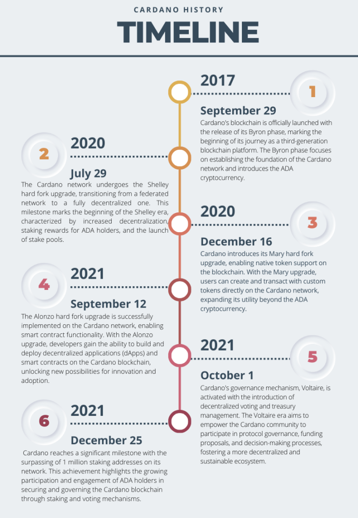
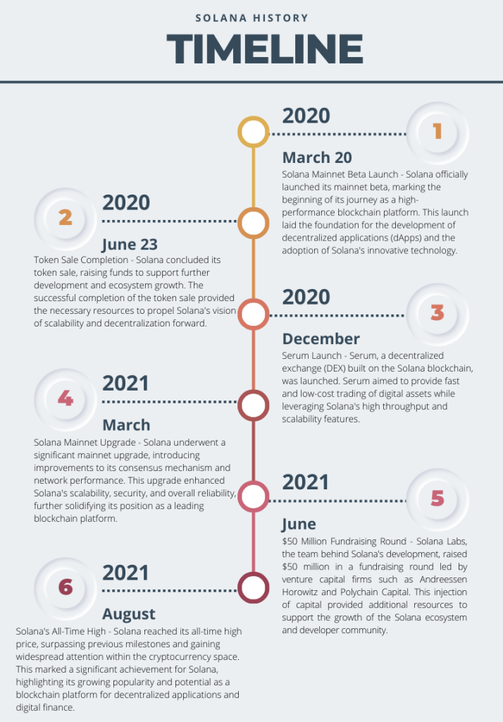
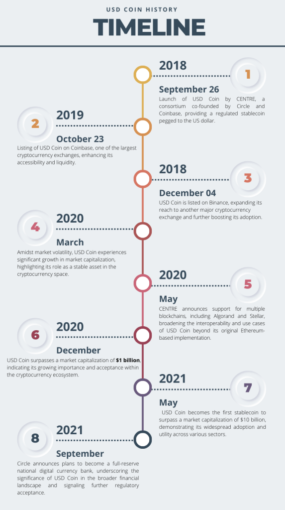
Figure 1. Key Dates in Cardano History
Source: Yahoo! Finance.
Key features
Layered Architecture
Cardano’s architecture is divided into two layers – the Cardano Settlement Layer (CSL) and the Cardano Computation Layer (CCL). This separation allows for greater flexibility, scalability, and easier implementation of updates and improvements.
Ouroboros Consensus Protocol:
Cardano uses the Ouroboros proof-of-stake consensus algorithm, which is designed to be secure, scalable, and energy-efficient. It allows users to participate in the consensus process based on the amount of cryptocurrency they hold, rather than requiring expensive computational resources.
Scalability
Cardano is designed to be highly scalable, capable of handling a large number of transactions per second. Through its layered architecture and consensus mechanism, Cardano aims to achieve scalability without sacrificing security or decentralization.
Interoperability
Cardano aims to enable interoperability between different blockchain networks and protocols. This will allow for seamless transfer of assets and data between different platforms, facilitating greater connectivity and usability of decentralized applications (dApps).
Smart Contracts
Cardano is developing support for smart contracts, which are self-executing contracts with the terms of the agreement directly written into code. Smart contracts will enable the creation of decentralized applications (dApps) on the Cardano platform, opening up a wide range of possibilities for developers and users.
Governance
Cardano has a built-in governance mechanism that allows stakeholders to participate in the decision-making process for the future development of the platform. This includes voting on proposals for protocol upgrades, funding development projects, and other governance-related decisions.
Formal Verification
Cardano emphasizes formal methods and peer-reviewed research in its development process. This includes using formal verification techniques to ensure the correctness and security of its protocols and smart contracts, reducing the risk of bugs and vulnerabilities.
Use cases
Decentralized Finance (DeFi)
Cardano’s smart contract capabilities can facilitate various DeFi applications, including decentralized exchanges (DEXs), lending platforms, stablecoins, and automated market makers (AMMs). Smart contracts on Cardano can enable programmable financial transactions without the need for intermediaries, providing users with greater control over their assets and reducing counterparty risk.
Supply Chain Management
Cardano’s blockchain can be utilized to track and authenticate products throughout the supply chain, ensuring transparency and accountability. By recording every step of a product’s journey on the blockchain, stakeholders can verify its origin, quality, and authenticity, thereby reducing fraud, counterfeiting, and logistical inefficiencies.
Identity Management
Cardano’s blockchain can serve as a secure and decentralized platform for identity management, enabling individuals to control and manage their digital identities without relying on centralized authorities. By leveraging cryptographic techniques, users can securely authenticate themselves and access various services, such as voting, healthcare, and financial transactions, while maintaining privacy and security.
Voting and Governance
Cardano’s blockchain can support transparent and tamper-resistant voting and governance systems, enabling communities to make collective decisions and govern decentralized organizations (DAOs). By using blockchain technology, voting processes can be made more secure, efficient, and auditable, ensuring fair and democratic outcomes.
Tokenization of Assets
Cardano’s blockchain can tokenize various real-world assets, such as real estate, stocks, and commodities, making them easily tradable and transferable on a global scale. By representing assets as digital tokens on the blockchain, ownership rights can be easily verified, fractional ownership can be enabled, and liquidity can be increased, unlocking new opportunities for investment and asset management.
Technology and Underlying Blockchain
Cardano is built on a multi-layered architecture designed to provide scalability, interoperability, and sustainability. At its core, Cardano utilizes a proof-of-stake (PoS) consensus mechanism called Ouroboros, which offers a more energy-efficient and secure alternative to traditional proof-of-work (PoW) systems. Ouroboros divides time into epochs and slots, with slot leaders responsible for creating new blocks and validating transactions within each slot. This approach ensures that the blockchain remains secure and decentralized while enabling high transaction throughput and low latency.
Cardano’s blockchain consists of two main layers: the Cardano Settlement Layer (CSL) and the Cardano Computation Layer (CCL). The CSL serves as the foundation for the platform’s native cryptocurrency, ADA, and facilitates secure and efficient peer-to-peer transactions. It employs a UTXO (Unspent Transaction Output) model similar to Bitcoin, where transactions are represented as inputs and outputs, ensuring transparency and immutability.
On top of the CSL, the CCL enables the execution of smart contracts and decentralized applications (dApps) using Plutus, Cardano’s purpose-built programming language. Plutus is based on Haskell, a functional programming language known for its safety and reliability, and allows developers to write smart contracts with formal verification capabilities, ensuring correctness and security. Additionally, Cardano supports interoperability with other blockchains through sidechains and cross-chain communication protocols, enabling seamless integration with existing infrastructure and networks.
Cardano’s development is guided by a rigorous scientific approach, with ongoing research and peer-reviewed papers driving innovation and advancement. The platform’s roadmap is divided into distinct phases, including Byron (foundation), Shelley (decentralization), Goguen (smart contracts), Basho (scaling), and Voltaire (governance), each focusing on specific features and functionalities. This modular approach allows for continuous improvement and evolution, ensuring that Cardano remains at the forefront of blockchain technology.
Supply of Coins
The supply of coins for Cardano (ADA) is governed by a predetermined protocol established during its initial launch. The total maximum supply of ADA is capped at 45 billion coins. Unlike some cryptocurrencies that have fixed supplies, Cardano’s distribution occurs gradually through a process called “minting.” During the initial phase, ADA tokens were distributed through a public sale and allocated to early supporters, development, and the Cardano treasury. Ongoing minting of ADA occurs through the process of staking, where ADA holders can delegate their coins to stake pools to participate in the network’s consensus and earn rewards. This incentivizes stakeholders to actively participate in the security and governance of the network while also distributing newly minted coins in a decentralized manner. As a result, the circulating supply of ADA gradually increases over time, with new coins being minted and distributed to participants in the Cardano ecosystem.
Historical data for Cardano
How to get the data?
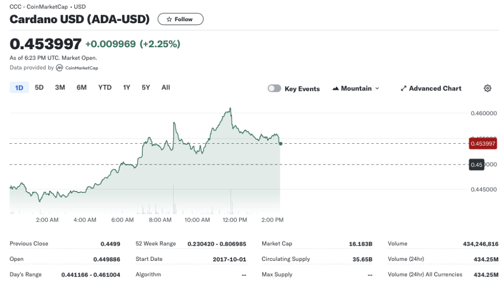
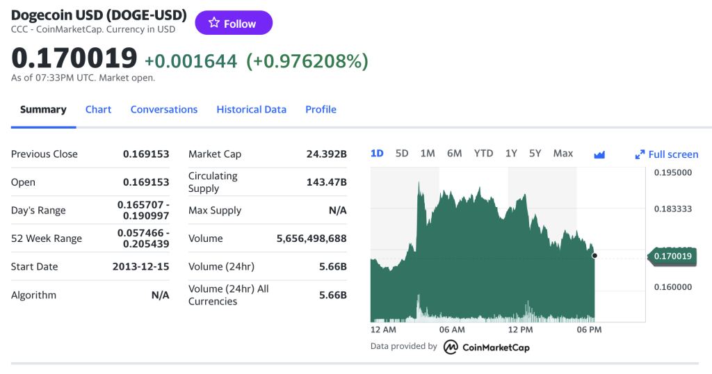
The Cordano is popular cryptocurrency on the market, and historical data for the Cordano such as prices and volume traded can be easily downloaded from the internet sources such as Yahoo! Finance, Blockchain.com & CoinMarketCap. For example, you can download data for Cardano on Yahoo! Finance (the Yahoo! code for Cardano is ADA-USD).
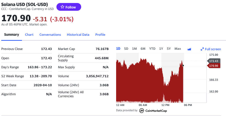
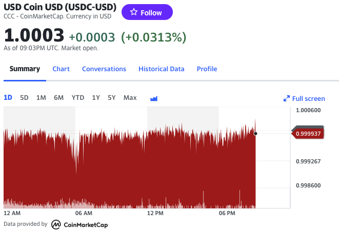
Figure 2. Cordano data
Source: Yahoo! Finance.
Historical data for the Cardano (ADA) market prices
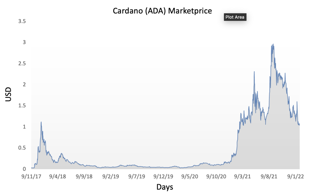
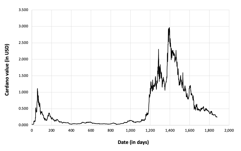
Cardano (ADA) has experienced notable fluctuations in its market price since its inception, reflecting both broader trends in the cryptocurrency market and developments specific to the Cardano project. Following its launch in 2017, ADA initially saw rapid growth, fueled by enthusiasm for its innovative technology and ambitious roadmap. However, like many cryptocurrencies, ADA’s price has been subject to volatility, with periods of sharp appreciation followed by corrections and consolidation. Historical data for Cardano’s market prices reveals a series of peaks and troughs, influenced by factors such as market sentiment, regulatory developments, technological milestones, and macroeconomic trends. Despite this volatility, Cardano has maintained its position as one of the top cryptocurrencies by market capitalization, attracting a dedicated community of supporters and investors. As the project continues to evolve and achieve key milestones, its market price remains closely watched by traders, investors, and stakeholders in the cryptocurrency ecosystem.
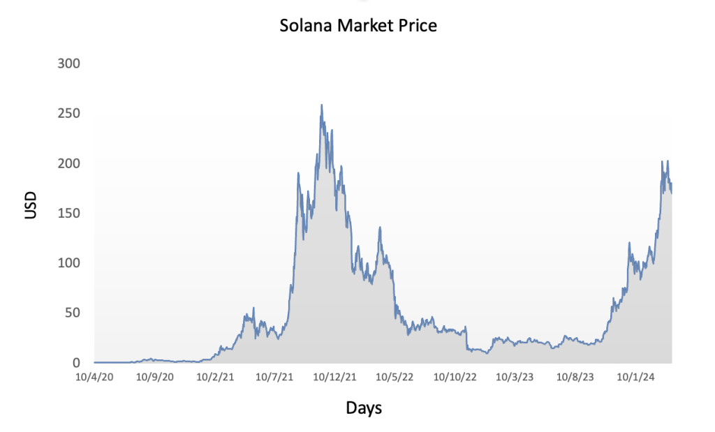
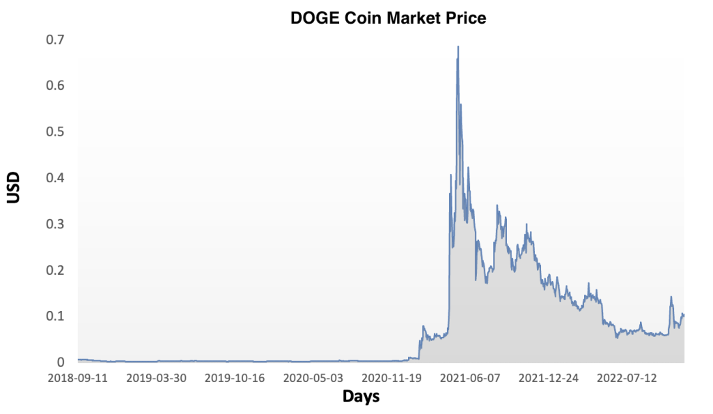
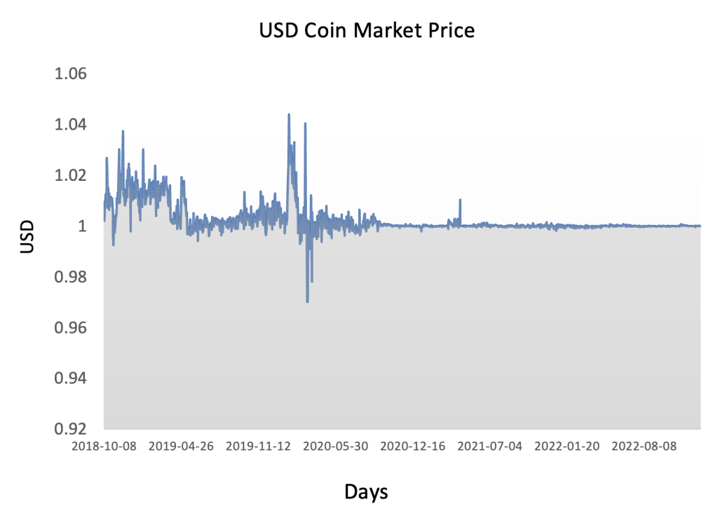
Figure 3 below represents the evolution of the price of Cardano (ADA) in US dollar over the period November 2017 – May 2024. The price corresponds to the “closing” price (observed at 10:00 PM CET at the end of the month).
Figure 3. Evolution of Cardano price
Source: Yahoo! Finance.
R program
The R program below written by Shengyu ZHENG allows you to download the data from Yahoo! Finance website and to compute summary statistics and risk measures about the Cardano (ADA).

Data file
The R program that you can download above allows you to download the data for the Cardano (ADA) from the Yahoo! Finance website. The database starts on November, 2017.
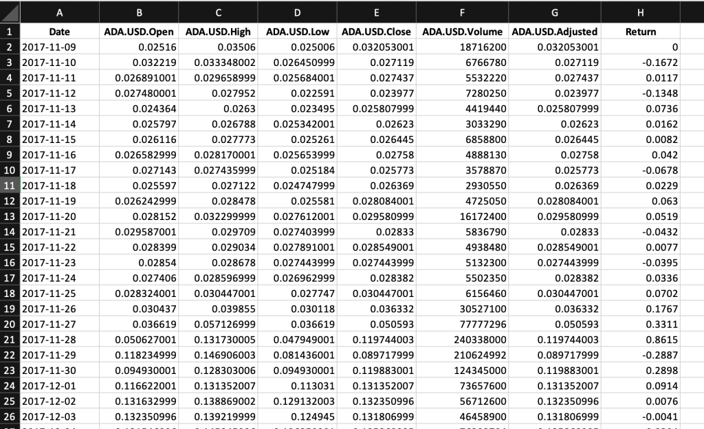
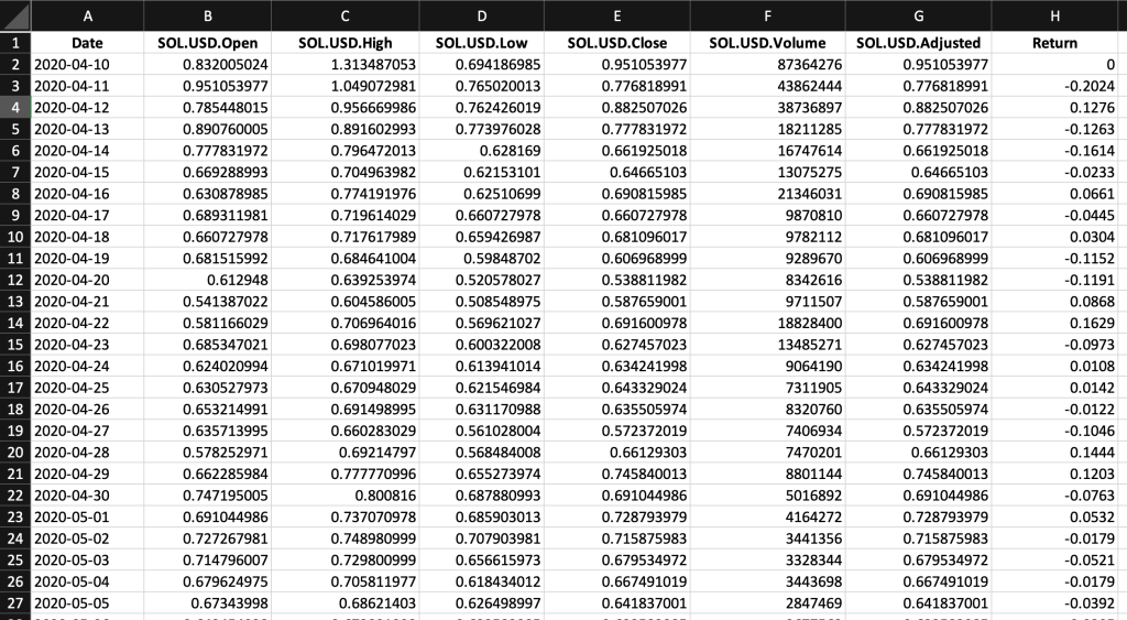
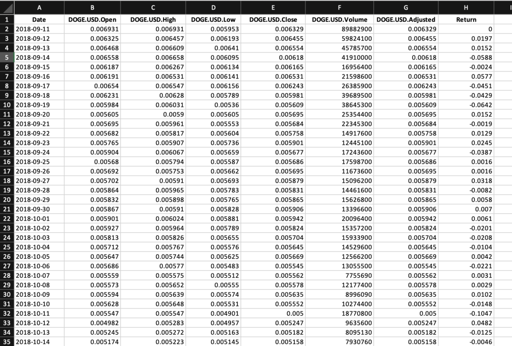
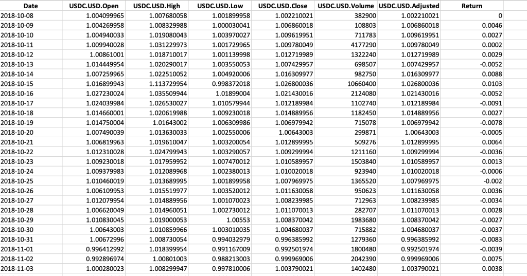
Table 1 below represents the top of the data file for the Cardano (ADA) downloaded from the Yahoo! Finance website with the R program.
Table 1. Top of the data file for the Cardano
Source: computation by the author (data: Yahoo! Finance website).
Python code
You can download the Python code used to download the data from Yahoo! Finance.

Python script to download Cardano (ADA) historical data and save it to an Excel sheet::
import yfinance as yf
import pandas as pd
# Define the ticker symbol for Cardano “ADA-USD”
Cardano_ticker = “ADA-USD”
# Define the date range for historical data
start_date = “2020-01-01”
end_date = “2022-01-01”
# Download historical data using yfinance
Cardano_data = yf.download(Cardano_ticker, start=start_date, end=end_date)
# Create a Pandas DataFrame from the downloaded data
Cardano_df = pd.DataFrame(Cardano_data)
# Define the Excel file path
excel_file_path = “Cardano _historical_data.xlsx”
# Save the data to an Excel sheet
Cardano_df.to_excel(excel_file_path, sheet_name=”Cardano Historical Data”)
print(f”Data saved to {excel_file_path}”)
# Make sure you have the required libraries installed and adjust the “start_date” and “end_date” variables to the desired date range for the historical data you want to download.
Evolution of the Cardano (ADA)
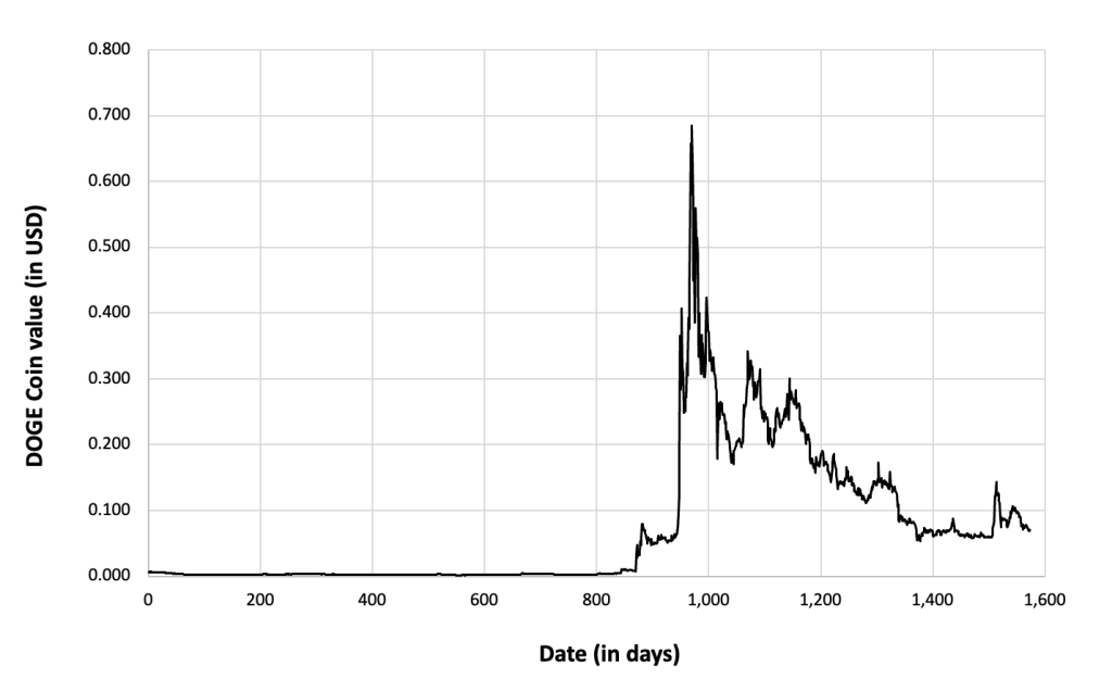
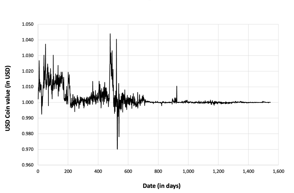
Figure 4 below gives the evolution of the Cardano (ADA) on a daily basis.
Figure 4. Evolution of the Cardano (ADA)
Source: computation by the author (data: Yahoo! Finance website).
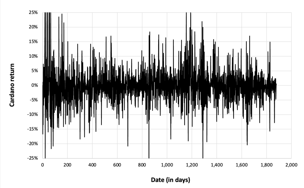
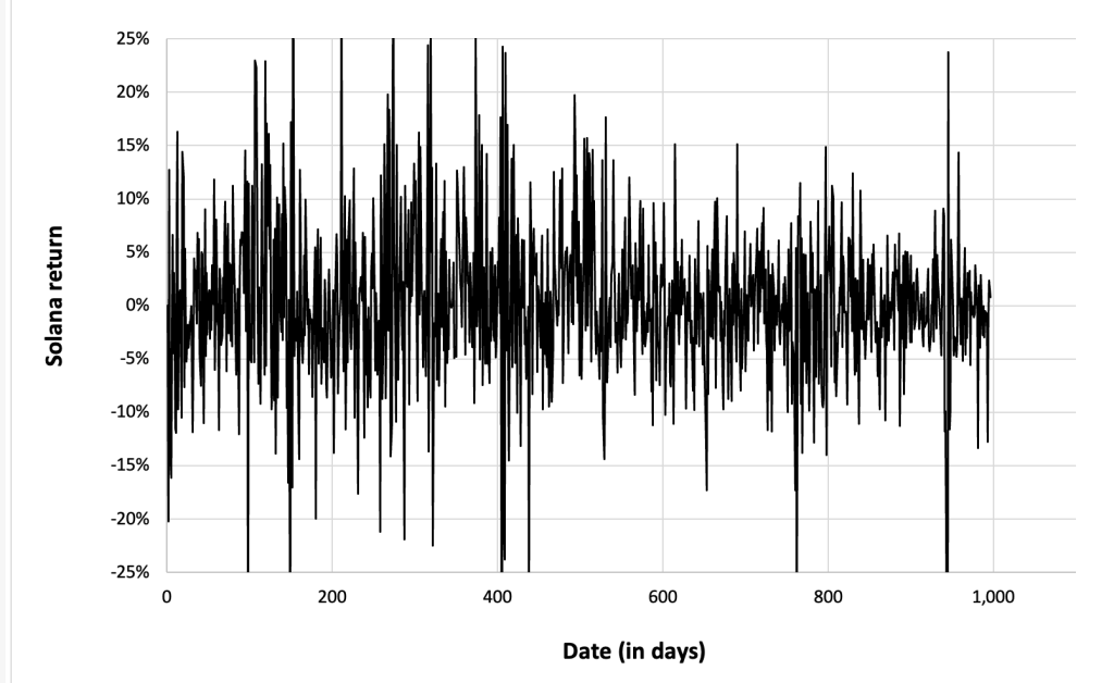
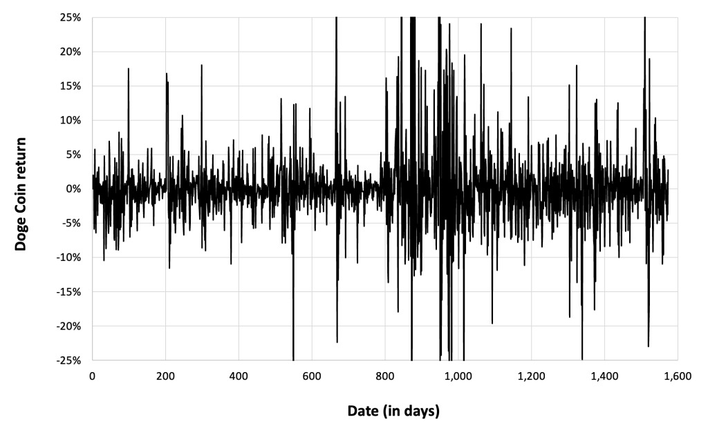
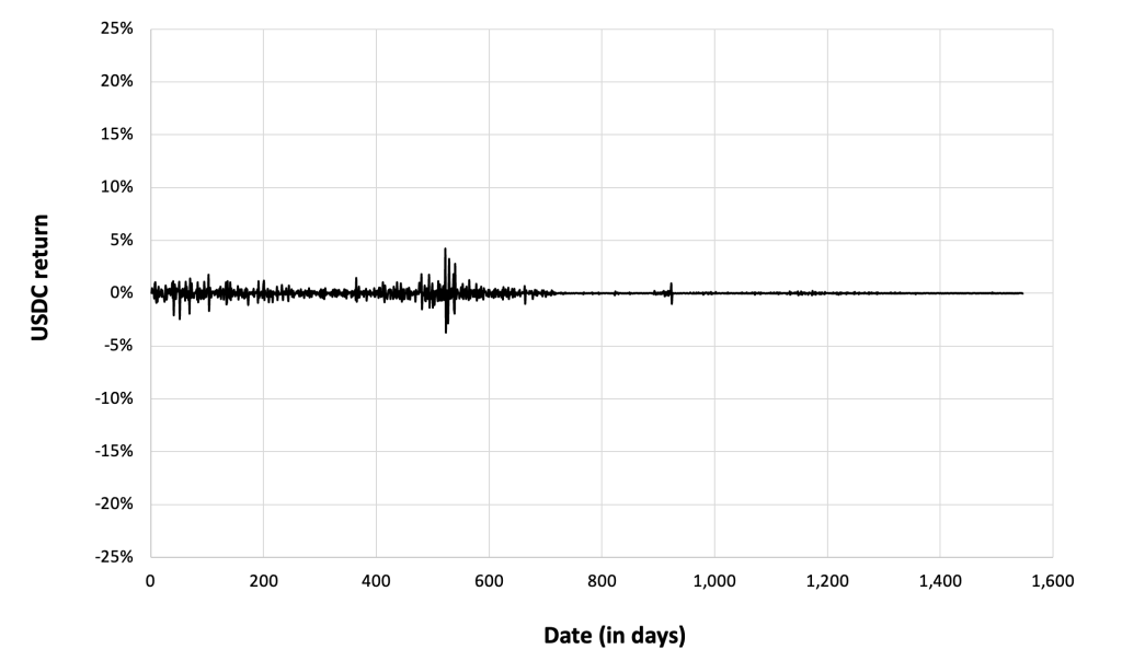
Figure 5 below gives the evolution of the Cardano (ADA) returns from November, 2017 to May, 2024 on a daily basis.
Figure 5. Evolution of the Cardano returns
Source: computation by the author (data: Yahoo! Finance website).
Summary statistics for the Cardano (ADA)
The R program that you can download above also allows you to compute summary statistics about the returns of the Cardano (ADA).
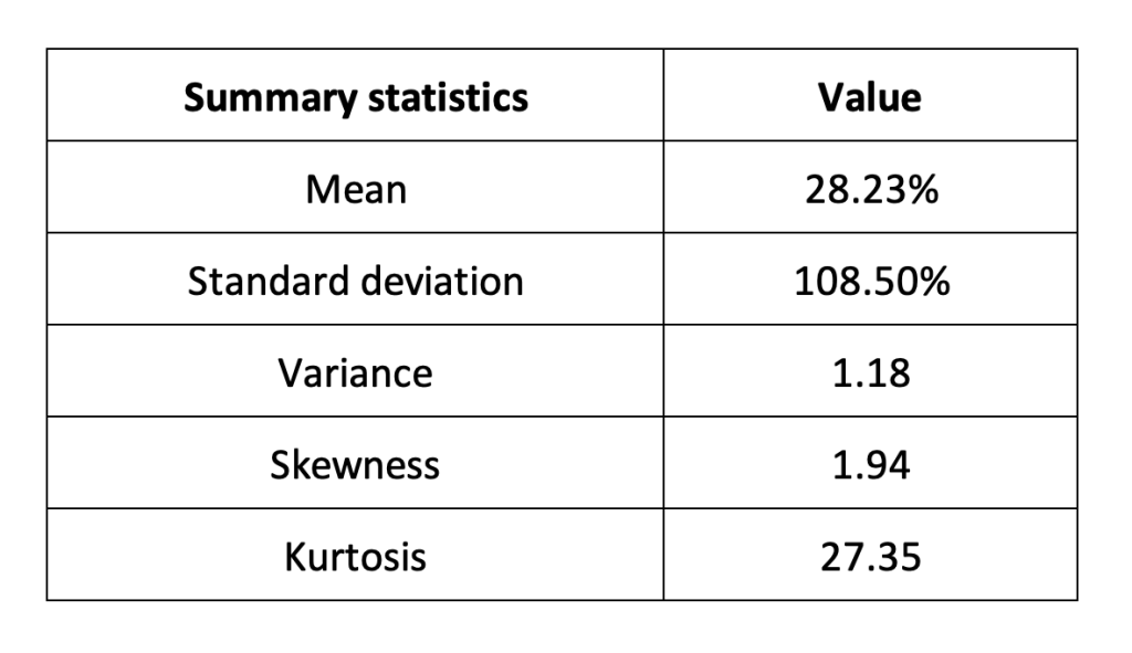
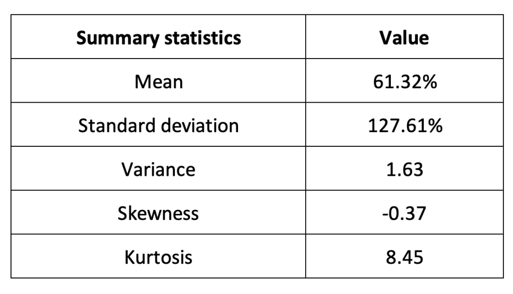
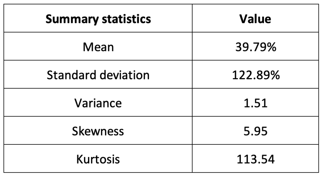
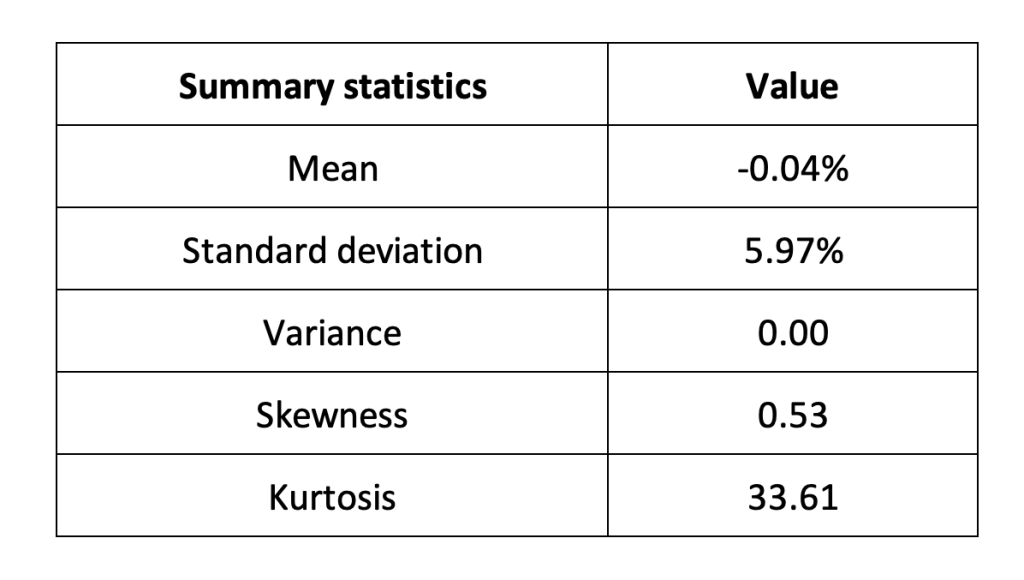
Table 2 below presents the following summary statistics estimated for the Cardano (ADA):
- The mean
- The standard deviation (the squared root of the variance)
- The skewness
- The kurtosis.
The mean, the standard deviation / variance, the skewness, and the kurtosis refer to the first, second, third and fourth moments of statistical distribution of returns respectively.
Table 2. Summary statistics for Cardano.
Source: computation by the author (data: Yahoo! Finance website).
Statistical distribution of the Cardano (ADA) returns
Historical distribution
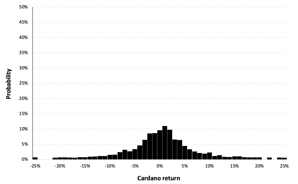
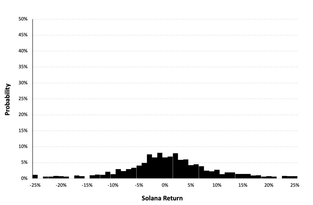
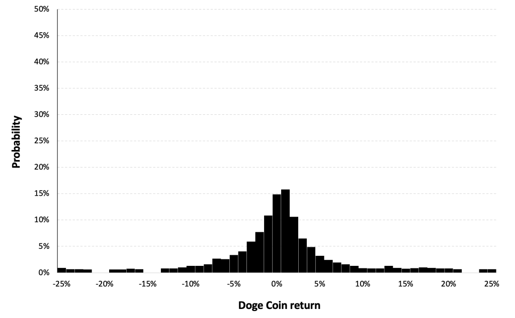
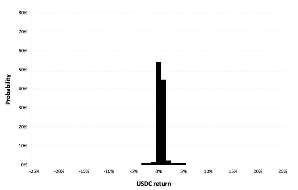
Figure 6 represents the historical distribution of the Cardano (ADA) daily returns for the period from November, 2017 to May, 2024.
Figure 6. Historical Cardano distribution of the returns.
Source: computation by the author (data: Yahoo! Finance website).
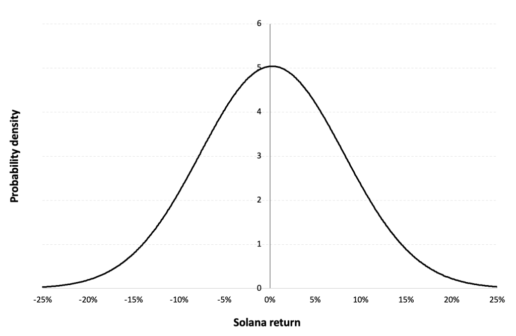
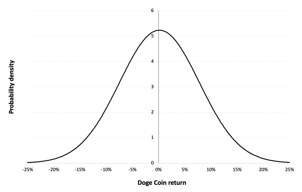
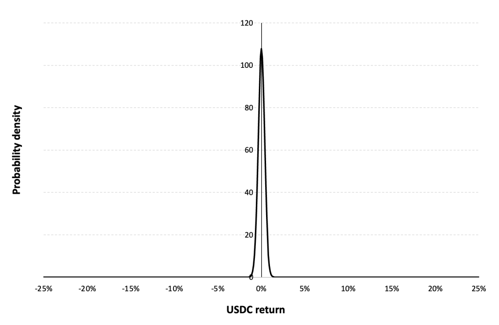
Gaussian distribution
The Gaussian distribution (also called the normal distribution) is a parametric distribution with two parameters: the mean and the standard deviation of returns. We estimated these two parameters over the period from November, 2017 to May, 2024.
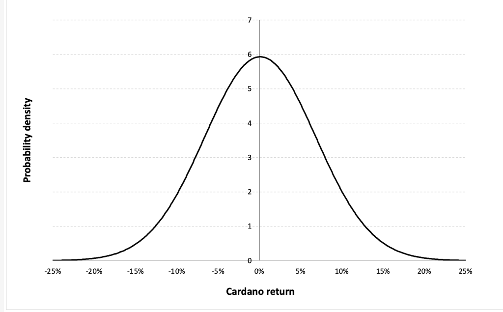
Figure 7 below represents the Gaussian distribution of the Ethereum daily returns with parameters estimated over the period from November, 2017 to May, 2024.
Figure 7. Gaussian distribution of the Cardano returns.
Source: computation by the author (data: Yahoo! Finance website).
Risk measures of the Cardano (ADA) returns
The R program that you can download above also allows you to compute risk measures about the returns of the Cardano (ADA).
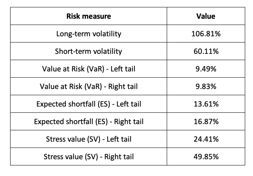
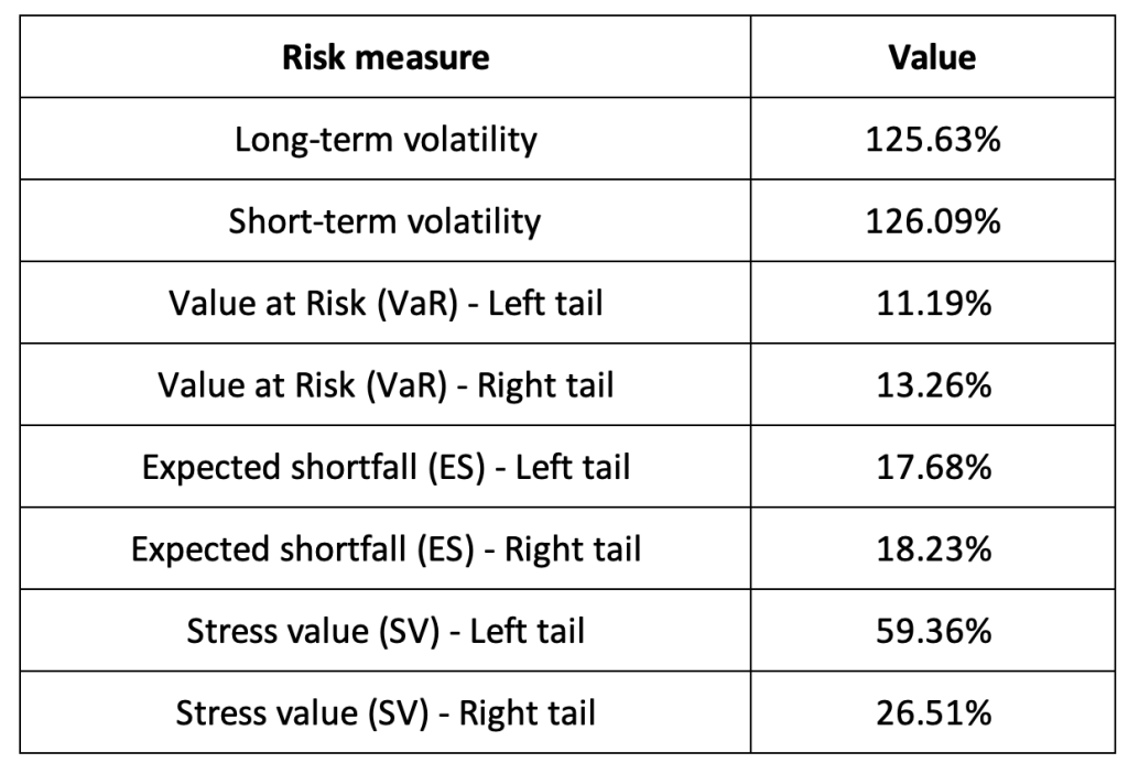
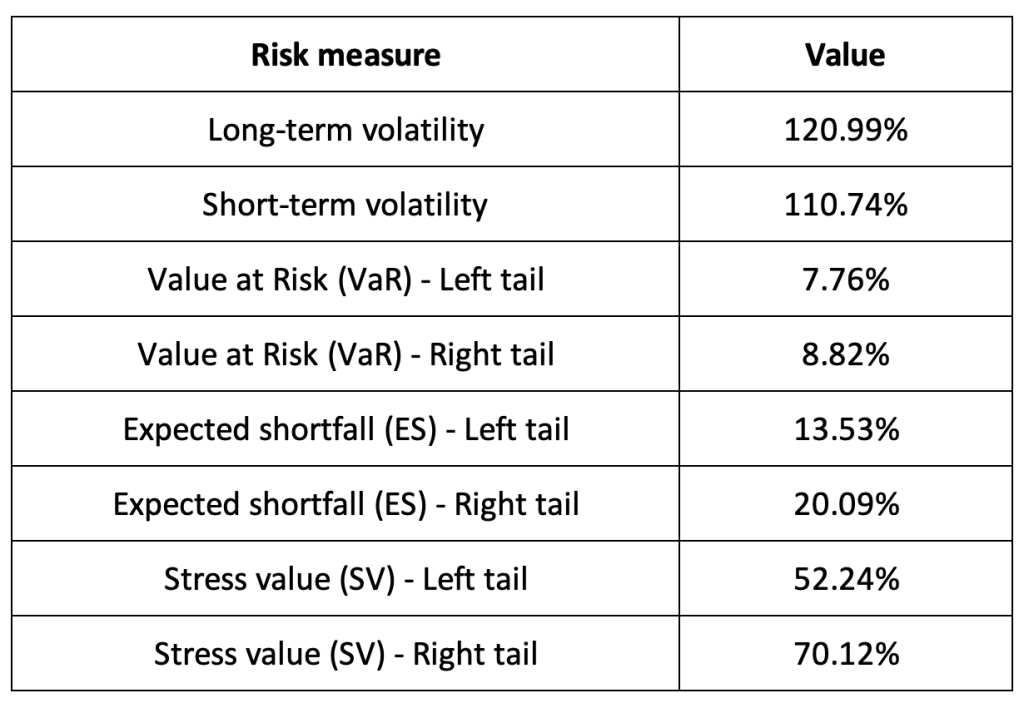
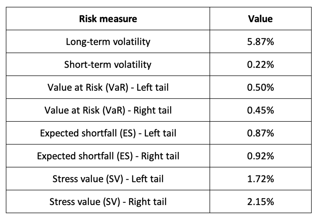
Table 3 below presents the following risk measures estimated for the Cardano (ADA):
- The long-term volatility (the unconditional standard deviation estimated over the entire period)
- The short-term volatility (the standard deviation estimated over the last three months)
- The Value at Risk (VaR) for the left tail (the 5% quantile of the historical distribution)
- The Value at Risk (VaR) for the right tail (the 95% quantile of the historical distribution)
- The Expected Shortfall (ES) for the left tail (the average loss over the 5% quantile of the historical distribution)
- The Expected Shortfall (ES) for the right tail (the average loss over the 95% quantile of the historical distribution)
- The Stress Value (SV) for the left tail (the 1% quantile of the tail distribution estimated with a Generalized Pareto distribution)
- The Stress Value (SV) for the right tail (the 99% quantile of the tail distribution estimated with a Generalized Pareto distribution)
Table 3. Risk measures for the Cardano.
Source: computation by the author (data: Yahoo! Finance website).
The volatility is a global measure of risk as it considers all the returns. The Value at Risk (VaR), Expected Shortfall (ES) and Stress Value (SV) are local measures of risk as they focus on the tails of the distribution. The study of the left tail is relevant for an investor holding a long position in the Cardano(ADA) while the study of the right tail is relevant for an investor holding a short position in the Cardano(ADA).
Why should I be interested in this post?
This post provides a compelling exploration of Cardano, catering to both novices and seasoned cryptocurrency enthusiasts alike. It delves into Cardano’s innovative blockchain technology and its role in revolutionizing various sectors, including finance, governance, and social impact initiatives. By understanding Cardano’s layered architecture, consensus mechanism, and ongoing development phases, readers can gain valuable insights into its potential to address scalability, interoperability, and sustainability challenges in the blockchain space. Moreover, the post examines Cardano’s historical performance, market dynamics, and community-driven governance model, offering invaluable perspectives for investors, traders, and stakeholders. Whether you’re intrigued by cutting-edge blockchain solutions or seeking investment opportunities in the cryptocurrency market, this post provides comprehensive insights into the significance and potential of Cardano in shaping the future of decentralized technologies.
Related posts on the SimTrade blog
About cryptocurrencies
▶ Snehasish CHINARA Bitcoin: the mother of all cryptocurrencies
▶ Snehasish CHINARA How to get crypto data
▶ Alexandre VERLET Cryptocurrencies
About statistics
▶ Shengyu ZHENG Moments de la distribution
▶ Shengyu ZHENG Mesures de risques
▶ Jayati WALIA Returns
Useful resources
Academic research about risk
Longin F. (2000) From VaR to stress testing: the extreme value approach Journal of Banking and Finance, N°24, pp 1097-1130.
Longin F. (2016) Extreme events in finance: a handbook of extreme value theory and its applications Wiley Editions.
Data
Yahoo! Finance
Yahoo! Finance Historical data for Cardano
CoinMarketCap Historical data for Cardano
About the author
The article was written in March 2024 by Snehasish CHINARA (ESSEC Business School, Grande Ecole Program – Master in Management, 2022-2024).