Capital Guaranteed Products

Capital Guaranteed Products

Shengyu ZHENG

In this article, Shengyu ZHENG (ESSEC Business School, Grande Ecole Program – Master in Management, 2020-2023) explains how capital guaranteed products are built.

Motivation for investing in capital-guaranteed products

In order to invest the surplus of the firm liquid assets, corporate treasurers take into account the following characteristics of the financial instruments: performance, risk and liquidity. It is a common practice that some corporate investment strategies require that the investment capital should at least be guaranteed. The sacrifice of this no-loss guarantee is limited return in case of appreciation of the underlying asset price.

Capital-guaranteed (or capital-protected) products are one of the most secure forms of investment, usually in the form of certificates. They provide a guarantee that a specified minimum amount (usually 100 per cent of the issuance price) will be repaid at maturity. They are suitable particularly for risk-averse investors who wish to hold the products through to maturity and are not prepared to bear any loss that might exceed the level of the guaranteed repayment.

Performance

Let us consider a capital-guaranteed product with the following characteristics:

Table 1. Characteristics of the capital-guaranteed products

Notional amount EUR 1,000,000.00
Underlying asset CAC40 index
Participation rate 40%
Minimum amount guarantee 100% of the initial level
Effective date February 01, 2022
Maturity date July 30, 2022

We also have the following information about the market:

Table 2. Market information

Risk-free rate (annual rate) 8%
Implied volatility (annualized) 10%

In case of depreciation of the underlying index, the return of the product remains zero, which means the original capital invested is guaranteed (or protected). In case of appreciation of the underlying index, the product only yields 40% of the return of the underlying index. The following chart is a straightforward illustration of the performance structure of this product.

Performance of the capital guaranteed product

Construction of a capital guaranteed product

We can decompose a capital-guaranteed product into three parts:

  • Investment in the risk-free asset that would yield the guaranteed capital at maturity
  • Investment in a call option that guarantees participation in the appreciation of the underlying asset
  • Margin of the bank

Decomposition of the capital guaranteed product

Investment in the risk-free asset

The essence of the capital guarantee is realized by investing a part of the initial capital in the risk-free asset and obtaining the amount of the guaranteed capital at maturity. Given the amount of the capital to be guaranteed and the risk-free rate, we can calculate the amount to be invested in risk-free asset: 1,000,000/(1+0.08)^0.5 =962,250.45 €

Investment in the call option

To realize the upside exposure, call options are a perfect vehicle. With a notional amount of 1,000,000 € and a maturity of 6 months, an at-the-money call option would cost 41,922.70 € (calculated with the Black-Scholes-Merton formula). Since the participation rate is 40%, the amount to be invested in the call option would be 16,769.08 € (= 40% * 41,922.70 €).

Margin of the bank

The margin of the bank is equal to the difference between the original capital and the two parts of the investment. In this case, the margin is 20,980.47 € (= 1,000,000.00 € – 962,250.45 € – 16,769.08 €)
If we compress the margin, there would be more capital available to invest in the call option, thus increasing the participation rate. In the case of zero margin, we obtain the maximum participation rate. In this scenario, the maximum participation rate would be 90.05% (= (1,000,000.00 € – 962,250.45 €) / 41,922.70 €).

Sensitivity to variations of the marketplace

Considering the two parts of the investment constituting the capital-guaranteed product, we can see that the risk-free rate and the volatility of the underlying asset are the two major factors influencing the pricing of this product. Here let us focus on the maximum participation rate as a proxy of the value of the product to the buyer of the product.

The effect of the risk-free rate could be ambiguous at the first glance. On one hand, if the risk-free rate rises, there needs to be less capital invested in the risk-free asset and there would be therefore more capital to be placed in purchasing the call options. On the other hand, if the risk-free rate rises, the call option value rises as well. With the same amount of capital, fewer call options could be purchased. However, the largest portion of the original capital is invested in the risk-free asset and the impact on this regard is more important. Overall, a rising risk-free rate has a positive impact on the participation rate.

The effect of the volatility of the underlying asset, however, is clear. Rising volatility has no impact on the risk-free investment in the framework of our hypotheses. It, however, raises the value of the call options, which means that fewer options could be purchased with the same amount of capital. Overall, rising volatility has a negative impact on the participation rate.

Statistical distribution of the return

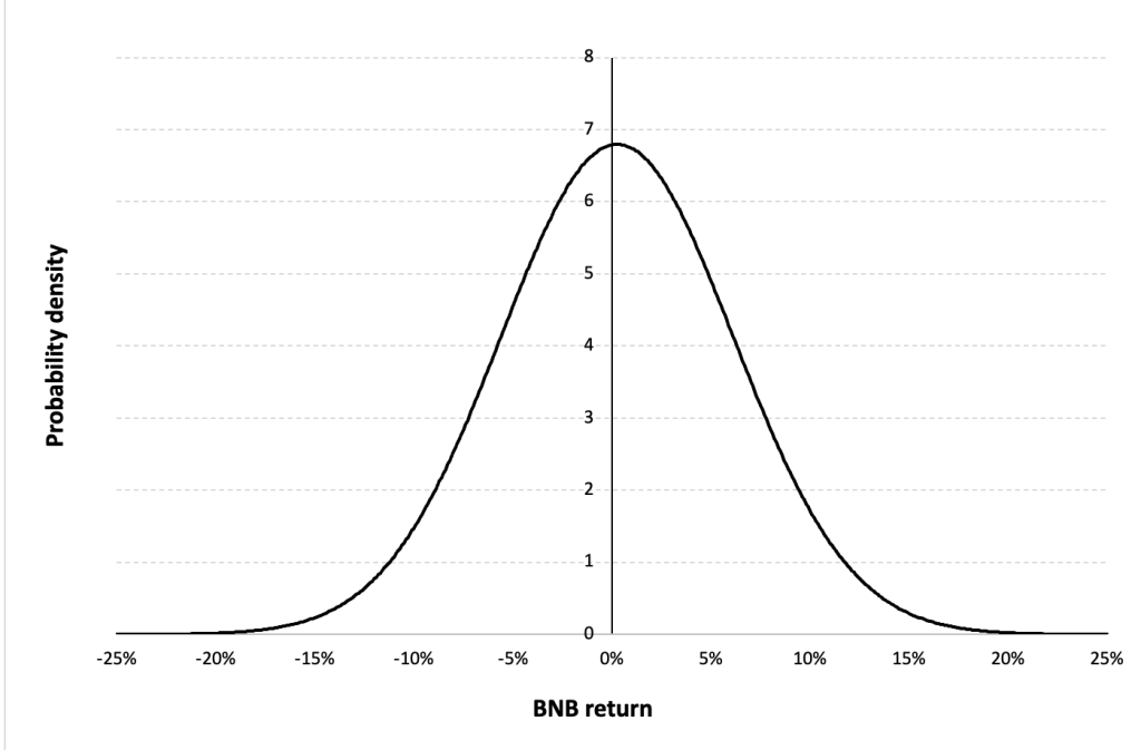
The statistical distribution of the return of the instrument is mixed by two parts: the discrete part equal to 0 corresponding to the case of depreciation of the underlying asset; and the continuous part of positive return. Based on a Gaussian assumption for the statistical distribution, we can calculate the probability mass of the depreciation of the underlying asset is 33.70%. In the continuous part, the return follows a Gaussian statistical distribution, with a mean equal to the periodic return over the participation rate and a standard deviation equal to periodic implied volatility over the participation rate, if the Gaussian assumption prevails.

Statistical distribution of the return of the capital guaranteed product

Risks and constraints

Liquidity risk

Being exotic financial instruments, capital-guaranteed products are not traded in standard exchanges. By construction, these products can normally only be redeemed at maturity and therefore are less liquid. There could be, however, early redemption clauses involved to mitigate the long-term liquidity risks. Investors should be aware of their liquidity needs before entering into a position in this product.

Counterparty risk

Similar to all other over-the-counter (OTC) transactions, there is no mechanism such as a central clearing counterparty (CCP) to ensure the timeliness and integrity of due payments. In case of financial difficulty including the bankruptcy of the issuer, the capital guarantee would be rendered worthless. It is therefore highly recommended to enter into such transactions with issuers of higher ratings.

Limited return

It is worth noting that capital-guaranteed products have weak exposure to the appreciation of the underlying asset. In this case, for a probability of 33.70%, there would be a return of zero, which is lower than investing directly in the risk-free security.

In order to mitigate this limit, the issuer could modify the level of guarantee to a lower level than 100%. This allows the product to have more exposure to the upside movement of the underlying asset with a relatively low risk of capital loss. To realize this involves entering positions of out-of-the-money call options.

Taxation and fees

In many countries, the return of capital-guaranteed products is considered as ordinary income, instead of capital gains or tax-advantaged dividends. For example, in Switzerland, it is not recommended to buy such a product with a long maturity, since the tax burden, in this case, could be higher than the “impaired” return of the product.

Moreover, fees for such products could be higher than exchange-traded funds (ETFs) or mutual funds. This part of investment cost should also be taken into account in making investment decisions.

Download the Excel file to analyze capital-guaranteed products

You can find below an Excel file to analyze capital-guaranteed products.

Download Excel file to analyze capital guaranteed products

Why should I be interested in this post?

As a family of investments that is often used in corporate treasury management, it is important to understand the mechanism and structure of capital-guaranteed products. It would be conducive for future asset managers, treasurer managers, or structurers to make the appropriate and optimal investment decisions.

Related posts on the SimTrade blog

   ▶ All posts about Options

   ▶ Shengyu ZHENG Barrier options

   ▶ Shengyu ZHENG Reverse convertibles

Resources

Books

Cox J. C. & M. Rubinstein (1985) “Options Markets” Prentice Hall.

Hull J. C. (2005) “Options, Futures and Other Derivatives” Prentice Hall, 6th edition.

Articles

Black F. and M. Scholes (1973) The Pricing of Options and Corporate Liabilities Journal of Political Economy, 81(3): 637-654.

Lacoste V. and Longin F. (2003) Term guaranteed fund management: the option method and the cushion method Proceeding of the French Finance Association, Lyon, France.

Merton R. (1974) On the Pricing of Corporate Debt Journal of Finance, 29(2): 449-470.

Websites

longin.fr Pricer for standard equity options – Call and put

Euronext www.euronext.com: website of the Euronext exchange where the historical data of the CAC 40 index can be downloaded

Euronext CAC 40 Index Option: website of the Euronext exchange where the option prices of the CAC 40 index are available

Six General information about capital protection without a cap: website of the Swiss stock exchange where information of various financial products are available.

About the author

The article was written in February 2023 by Shengyu ZHENG (ESSEC Business School, Grande Ecole Program – Master in Management, 2020-2023).

My Internship Experience at AlixPartners in London

My Internship Experience at AlixPartners in London

Federico De ROSSI

In this article, Federico De Rossi (ESSEC Business School, Master in Strategy and Management of International Business, 2020-2023) shares his professional experience as Business Analyst Intern at AlixPartners.

About the company

AlixPartners is a global consulting firm that offers companies facing complex challenges strategic, operational, and financial advice. They collaborate with companies in a variety of industries, including automotive, consumer goods, healthcare, retail, and technology. The company was founded in 1981 in Detroit, Michigan, and has since expanded to become a global firm with offices in more than 25 countries.

Logo of the AlixPartner.
Logo of AlixPartner
Source: AlixPartner.

My internship

During my internship at AlixPartners, I worked as a Business Analyst Intern.

My missions

My role was twofolded: on one side I was involved in providing support to consultants all over the globe on various projects and different industries. On the other side, I also worked hand to hand with the firm’s managing director to spot business development opportunities by, for instance, analysing four of the biggest private equity firms in the world and their portfolio companies.

Finally, I was responsible for conducting research and analysis to support project work, preparing presentations and reports for clients, and attending team meetings.

Required skills and knowledge

As an Intern in a global consulting firm, I already had to master some skills that would have been necessary for a successful completion of the internship itself. Obviously, learning agility and curiosity are given qualities that candidates are asked to have: without them, working 10+ hours a day would not be sustainable and would not make the job interesting. On top of those, problem-solving and communication skills are the bread and butter of the industry. Finally, for what concerned hard skills, a good knowledge of the Microsoft Office suite was fundamental.

What I learned

My internship at AlixPartners provided me with a valuable learning experience. It helped me develop a range of skills, including problem-solving, analytical, and communication skills. I also learned the importance of teamwork, collaboration, and time management.

One of the key things that I learned during my internship was the importance of developing a deep understanding of the client’s business. This involved analyzing the client’s financial statements, conducting market research, and understanding their competitive landscape. This understanding helped consulting firms develop customized solutions that are tailored to the client’s specific needs.

Another valuable lesson that I learned was the importance of effective communication. As consultants, we had to present our findings and recommendations to clients in a clear and concise manner. This involved preparing presentations and reports that were easy to understand and conveyed the key messages effectively.

Finally, working in such a high paced environment, with long hours and very demanding challenges, I definitely learnt how to better manage my time and conciliate my personl life with my professional one.

Financial concepts related my internship

When it comes to financial concepts related to the industry, I haven’t been exposed to much if not for when I had to analyze private equity firms such as KKR, Bain Capital, EQT, and others. It was the first time I was working on PEs and the topic revealed itself to be extremely enjoyable. It’s quite interesting to see the deep connection between private equity and consulting.

Why should I be interested in this post?

Overall, my internship at AlixPartners was a fantastic learning opportunity that enabled me to develop a variety of skills that will be useful in my future career. I would strongly recommend AlixPartners to anyone interested in a career in consulting.

Related posts on the SimTrade blog

   ▶ All posts about professional experience

   ▶ Nithisha CHALLA My experience as a Risk Advisory Analyst in Deloitte

   ▶ Alexandre VERLET My experience as an investment banking analyst intern at G2 Capital Advisors

Useful resources

AlixPartner

About the author

The article was written in March 2022 by Federico De Rossi (ESSEC Business School, Master in Strategy and Management of International Business, 2020-2023).

Understanding the Order Book: How It Impacts Trading

Understanding the Order Book: How It Impacts Trading

Federico De ROSSI

In this article, Federico DE ROSSI (ESSEC Business School, Master in Strategy & Management of International Business (SMIB), 2020-2023) talks about the order book and explains its role in financial markets.

Introduction

Understanding the order book is critical when it comes to trading in financial markets. In this article, we’ll go over what an order book is and how it affects trading.

What is an order book?

An order book for a stock, currency, or cryptocurrency is a list of buy and sell limit orders for that asset. It shows the pricing at which buyers and sellers are willing to negotiate, as well as the total number of orders available at each price. The order book is a necessary component of every trading platform since it gives a snapshot of the current market situation, of the price of the assets, and of the liquidity of the market. Thus, it is a crucial tool for traders who want to make informed decisions when entering or exiting deals.

How does an order book work?

The order book is a constantly updated record of buy and sell orders. When a trader puts a limit order, it is placed in the order book at the stated price. As a result, there is a two-sided market with distinct prices for buyers and sellers.

The order book is divided into two sections: bid (buy) and ask (sell). All open buy orders are displayed on the bid side, while all open sell orders are displayed on the ask side. The order book also shows the total volume of buy and sell orders at each price level.

In Tables 1 and 2 below, we give below two examples of order book from online brokers. We can see the two parts of the order book side by side: the “Buy” part and the “Sell” part. Every line of the order book corresponds to a buy or sell proposition for a give price (“Buy” or “Sell” columns) and a given quantity (“Volume” columns). For a given line there may be one or more orders for the same price. When there are several orders, the quantity in the “Volume” column is equal to the sum of the quantities of the different orders. Associated to the order book, there is often a chart which indicates the cumulative quantity of the orders in the order book at a given price. This chart gives an indication of the liquidity of the market in terms of market spread, market breadth, and market depth (see below for more explanations about theses concepts).

The “Buy” and “Sell” parts of the order book can be presented side by side (Table 1) or above each other (Tables 2 and 3) with the “Sell” part (in red) above the “Buy” part (in green) as the price limits of the sell limit orders are always higher than the price limits of the buy limit orders.

Table 1. Example of an order book (buy and sell parts presented side by side).
Order book
Source: online broker (Fortuneo).

Table 2. Example of an order book (buy and sell parts presented above each other).
Order book
Source: online broker (Cryptowatch).

Table 3. Example of an order book (buy and sell parts presented next to each other).
Order book
Source: online broker (Binance).

In a typical order book, the buy side is organized in descending order, meaning that the highest buy orders (i.e., the orders with the highest bid prices) are listed first, followed by the lower buy orders in descending order of price. The highest buy order in the book represents the best bid price, which is the highest price that any buyer is currently willing to pay for the asset.

On the other side of the order book, the sell side is organized in ascending order, with the lowest sell orders (i.e., the orders with the lowest ask prices) listed first, followed by the higher sell orders in ascending order of price. The lowest sell order in the book represents the best ask price, which is the lowest price that any seller is currently willing to accept for the asset.

This organization of the order book makes it easy for traders to see the current market depth and the best available bid and ask prices for an asset. When a buy order is executed at the best ask price or a sell order is executed at the best bid price, the order book is updated in real-time to reflect the new market depth and the new best bid and ask prices.

Table 4 below represents how the order book (limit order book) in trading simulations the SimTrade application.

Table 4. Order book in the SimTrade application.
Order book in the SimTrade application

You can understand how the order book works by launching a trading simulation on the SimTrade application.

The role of the order book in trading

As mentioned before, the order book is incredibly significant in trading. It acts as a market barometer, delivering real-time information about the supply and demand for an asset. Traders can also use the order book to determine market sentiment. If the bid side of the order book is strongly occupied, for example, it could imply that traders are optimistic on the asset. Thanks to the data in the order book, traders can get different information out of it.

Three characteristics of the order book

Market spread

The market spread, also known as the bid-ask spread, is the difference between the highest price a buyer is willing to pay for an asset (the bid price) and the lowest price a seller is willing to accept (the ask price) at a particular point in time.

The market spread is a reflection of the supply and demand for the asset in the market, and it represents the transaction cost of buying or selling the asset. In general, a narrow or tight spread indicates a liquid market with a high level of trading activity and a small transaction cost, while a wider spread suggests a less liquid market with lower trading activity and a higher transaction cost.

Market breadth

Market breadth is a measure of the overall health or direction of a market, sector, or index. It refers to the number of individual stocks that are participating in a market’s movement or trend, and can provide insight into the underlying strength or weakness of the market.

Market breadth is typically measured by comparing the number of advancing stocks (stocks that have increased in price) to the number of declining stocks (stocks that have decreased in price) over a given time period. This ratio is often expressed as a percentage or a ratio, with a higher percentage or ratio indicating a stronger market breadth and a lower percentage or ratio indicating weaker breadth.

For example, if there are 1,000 stocks in an index and 800 of them are increasing in price while 200 are decreasing, the market breadth ratio would be 4:1 or 80%. This would suggest that the market is broadly advancing, with a high number of stocks participating in the upward trend.

Market depth

Finally, market depth is a measure of the supply and demand of a security or financial instrument at different prices. It refers to the quantity of buy and sell orders that exist at different price levels in the market. Market depth is typically displayed in a market depth chart or order book.

It can provide valuable information to traders and investors about the current state of the market. A deep market with large quantities of buy and sell orders at various price levels can indicate a liquid market where trades can be executed quickly and with minimal impact on the market price. On the other hand, a shallow market with few orders at different price levels can indicate a less liquid market where trades may be more difficult to execute without significantly affecting the market price.

Analyzing order book data

Data from order books can be used to gain insight into market sentiment and trading opportunities. For example, traders can use the bid-ask spread to determine an asset’s liquidity. They can also examine the depth of the order book to determine the level of buying and selling interest in the asset. Traders can also use order book data to identify potential trading signals. For example, if the bid side of the order book is heavily populated at a certain price level, this could indicate that the asset’s price is likely to rise. On the other hand, if the ask side is heavily populated at a certain price level, it could indicate that the asset’s price is likely to fall.

Benefits of using order book data for trading

Using order book data can provide traders with a number of advantages.

For starters, it can be used to gauge market sentiment and identify potential trading opportunities.

Second, it can assist traders in more effectively managing risk. Traders can identify areas of support and resistance in order book data, which can then be used to set stop losses and take profits.

Finally, it can aid traders in the identification of potential trading signals. Traders can identify areas of potential buying and selling pressure in order book data, which can then be used to enter and exit trades.

How to use order book data for trading

Traders can use order book data to gain a competitive advantage in the markets. To accomplish this, they must first identify areas of support and resistance that can be used to set stop losses and profit targets.

Traders should also look for indications of buying and selling pressure in the order book. If the bid side of the order book is heavily populated at a certain price level, it could indicate that the asset’s price is likely to rise. On the other hand, if the ask side is heavily populated at a certain price level, it could indicate that the asset’s price is likely to fall.

Finally, traders should use trading software to automate their strategies. Trading bots can be set up to monitor order book data and execute trades based on it. This allows traders to capitalize on trading opportunities more quickly and efficiently.

Conclusion

To summarize, the order book is a vital instrument for financial market traders. It gives real-time information about an asset’s supply and demand, which can be used to gauge market mood and find potential trading opportunities. Traders can also utilize order book data to create stop losses and take profits and to automate their trading techniques. Traders might obtain an advantage in the markets by utilizing the power of the order book.

Related posts on the SimTrade blog

▶ Jayna MELWANI The impact of market orders on market liquidity

▶ Lokendra RATHORE Good-til-Cancelled (GTC) order and Immediate-or-Cancel (IOC) order

▶ Clara PINTO High-frequency trading and limit orders

▶ Akshit GUPTA Analysis of The Hummingbird Project movie

Useful resources

SimTrade course Trade orders

SimTrade course Market making

SimTrade simulations Market orders   Limit orders

About the author

The article was written in March 2023 by Federico DE ROSSI (ESSEC Business School, Master in Strategy & Management of International Business (SMIB), 2020-2023).

The Power of Patience: Warren Buffett's Advice on Investing in the Stock Market

The Power of Patience: Warren Buffett’s Advice on Investing in the Stock Market

Federico De ROSSI

In this article, Federico De ROSSI (ESSEC Business School, Master in Strategy and Management of International Business, 2020-2023) comments on a quote by Warren Buffet about patience.

Quote

The stock market is a device for transferring money from the impatient to the patient.

Analysis of the quote

The quote “The stock market is a device for transferring money from the impatient to the patient” was written by none other than Warren Buffett, widely regarded as one of the greatest investors of all time. Buffett is the chairman and CEO of Berkshire Hathaway, a multinational conglomerate holding company with a diverse portfolio of businesses in insurance, energy, railroads, manufacturing, and retail. As of the 2nd of March 2023, the oracle of Omaha has amassed a net worth of more than $100 billion over the course of his career, owing largely to his astute stock market investments. Buffett’s investment philosophy revolves around identifying high-quality companies with strong competitive advantages and investing in them for the long term, often with a holding period of 10 years or even more. A strategy also known as value investing.

Financial concepts related to the quote

Related to this quote, I spotted three main financial concepts: compounding returns, long-term investment strategy, and risk and reward.

Compounding returns

One of the financial concepts associated with Buffett’s quote is the idea of compounding returns. Essentially, the longer you hold onto a stock, the more money you stand to make. By reinvesting your earnings and letting them compound over time, you can potentially turn a small initial investment into a large sum of money over the course of several years or even decades. This is where patience comes in – if you’re constantly buying and selling stocks, you’re unlikely to see the full benefits of compounding returns.

Long-term investment strategy

Another concept that ties into Buffett’s quote is the importance of having a long-term investment strategy. The stock market can be incredibly volatile in the short-term, with prices fluctuating wildly based on a variety of factors such as news events, economic data, and investor sentiment. However, over the long-term, the stock market tends to follow a generally upward trend, as companies grow and earnings increase. By having a long-term investment strategy and holding onto your stocks through market fluctuations, you can avoid making rash decisions based on short-term movements and instead focus on the bigger picture.

Risk and reward

A third financial concept related to Buffett’s quote is the idea of risk and reward. The higher the potential reward, the higher the level of risk involved. Stocks with high growth potential may offer greater returns, but they also come with greater risk of volatility and price fluctuations. On the other hand, more stable, established companies may offer lower returns but come with lower risk. By being patient and willing to wait for your investments to pay off over the long-term, you can potentially reap the rewards of higher returns while minimizing your risk.

My opinion about this quote

In my opinion, Buffett’s quote is a testament to the power of patience and long-term thinking when it comes to investing. Too often, people are tempted to make quick, impulsive decisions based on short-term market movements or the latest hot stock tip. However, this approach rarely leads to long-term success. Instead, by taking a patient, disciplined approach to investing and focusing on high-quality companies with strong fundamentals, you can potentially build wealth over the course of years or even decades. While investing in the stock market always involves some level of risk, by being patient and letting your investments compound over time, you can potentially reap the rewards of higher returns and build a more secure financial future.

Why should I be interested in this post?

This quote is a great reminder to always invest money with your brain and not based on your emotions. Be patient – fools rush in where angels fear to tread.

Related posts on the SimTrade blog

   ▶ All posts about Quotes

   ▶ Akshit GUPTA Warren Buffett – The Oracle of Omaha

   ▶ Youssef LOURAOUI Long-short equity strategy

   ▶ Rayan AKKAWI Warren Buffet and his basket of eggs

   ▶ Youssef EL QAMCAOUI The Warren Buffett Indicator

Useful resources

Berkshire Hathaway

About the author

The article was written in March 2023 by Federico De ROSSI (ESSEC Business School, Master in Strategy and Management of International Business, 2020-2023).

The Islamic financial system as a solution to tackle social issues

The Islamic financial system as a solution to tackle social issues

Evan CHAISSON

In this article, Evan CHAISSON (ESSEC Business School, Master in Strategy & Management of International Business (SMIB), 2022-2023) comments on a quote by Wolfgang Schafuble about Islamic finance.

Quote

Islamic finance is growing in importance for the global economy. It is therefore important consider questions related to integrating Islamic finance into global finance.

Analysis of the quote

This quote, by Wolfgang Schauble, highlights the growing importance of Islamic finance in the global economy. Islamic finance is a rapidly growing sector, with an estimated value of over $2 trillion in assets worldwide. Figure 1 below gives the Global Islamic Finance Assets Growth (in US$ Trillions). As you can see from the figure, the sector is projected to more than double in value in 2024 based on its 2012 value.

Figure 1. Global Islamic Finance Assets Growth.
Global Islamic Finance Assets Growth
Source: ICD – Refinitiv Islamic Finance Development Report (December 2020).

As such, it is becoming increasingly important for the global financial system to consider questions related to integrating Islamic finance into global finance.

Additionally, this quote presents Islamic finance as a financial system that is different from the classical “Western” system that is commonplace today. As such, it may be able to offer solutions to global issues that the current system is unable to solve.

About the author

Wolfgang Schauble is a German politician who has played a prominent role in German and European politics for several decades. He served as Germany’s Minister of Finance from 2009 to 2017, during which time he played a key role in managing the global financial crisis and the European debt crisis.

Prior to serving as Minister of Finance, Schauble served as Minister of the Interior, where he was responsible for domestic security and law enforcement. He is widely regarded as a conservative politician and has been a member of the Christian Democratic Union (CDU) since 1974.

Financial concepts related to the quote

Although much separates Islamic law from the Western system, there are three main aspects that stand out: prohibition of interest, asset-based financing, and ethical and social considerations.

Prohibition of interest

The prohibition of interest, or riba, is one of the foundational principles of Islamic finance. This principle is based on the Islamic belief that money should not be used as a commodity to generate profit. The concept of riba is not limited to charging interest on loans, but also includes any type of fixed, predetermined, or guaranteed return on investment. Instead of interest-based lending, Islamic finance relies on profit-and-loss sharing (PLS) arrangements, where both the lender and the borrower share the risks and rewards of a particular investment.

PLS contracts take several forms, including mudarabah, musharakah, and ijara. In mudarabah, one party provides the capital, and the other party provides the expertise to invest the capital. Profits are shared according to a pre-agreed ratio, but losses are borne solely by the provider of capital. In musharakah, both parties provide capital and expertise, and profits and losses are shared according to a pre-agreed ratio. In ijara, the financier purchases an asset and leases it to the borrower for a fixed period of time, with the option to purchase the asset at the end of the lease term.

Asset-based financing

In Islamic finance, financial investments are tied to physical assets, such as property or commodities, rather than financial instruments such as stocks, bonds, or, say mutual funds. This is known as asset-based financing, and it is designed to promote stability in the financial system. By tying financial investments to tangible, physical assets, Islamic finance encourages investment in the real economy and discourages speculation.

The use of asset-based financing also has implications for risk management. Since investments are tied to real assets, the risks associated with those investments are more tangible and can be more easily managed. This also encourages all parties involved to share the risk of the venture. In turn, this will help build trust between partners, and, as more time goes by, investment risk will steadily decrease.

Ethical and social considerations

Islamic finance places a strong emphasis on ethical and social considerations in investment decisions. This includes avoiding investments in industries such as alcohol, tobacco, and gambling, which are considered harmful to society. Additionally, Islamic finance institutions often have social welfare programs that aim to promote social justice and alleviate poverty.

One example of a social welfare program in Islamic finance is zakat, which is a form of mandatory charitable giving. Muslims are required to give a portion of their wealth to those in need, and Islamic finance institutions often collect and distribute zakat on behalf of their clients. Islamic finance institutions may also engage in other forms of social welfare, such as providing interest-free loans to small businesses or supporting community development projects.

My opinion about this quote

Having stumbled on this quote by chance, I chose it because it made me curious about a financial system which I previously was not familiar with. This then led me to learn about a financial system which operates in a way that is decidedly different from what Westerners are used to. As a young adult growing up in an increasingly uncertain world with more than its fair share of issues, I am always searching for a solution. Thanks to this quote, I have discovered a financial system that, perhaps, can shape a path towards a better future.

Why should I be interested in this post?

Any student of business and finance, regardless of its origins, has much to gain from simply learning about the Islamic financial system.

This system should be studied, first and foremost, simply because Islamic finance is an increasingly important and influential component of the global financial system. According to the Islamic Financial Services Board, the global Islamic finance industry had assets worth $2.88 trillion in 2019. As the industry continues to grow, there will be a growing demand for professionals who understand the principles and practices of Islamic finance.

Another more ethical reason is because, as mentioned earlier, Islamic finance places a strong emphasis on ethical and social considerations in investment decisions. This includes avoiding investments in industries such as alcohol, tobacco, and gambling, which are considered harmful to society. For students who are interested in pursuing careers in finance with a social and ethical focus, Islamic finance may be of particular interest.

Related posts on the SimTrade blog

   ▶ All post about Quotes

   ▶ Paul Antoine BOHOUN Bourse Régionale des Valeurs Mobilières

Useful resources

Islamic Finance: Principles, Performance and Prospects

About the author

The article was written in March 2023 by Evan CHAISSON (ESSEC Business School, Grande Ecole – Master in Strategy & Management of International Business, 2022-2023).

How to choose an online broker to invest in the stock market

How to choose an online broker to invest in the stock market

In reality, individuals cannot directly access the market to buy or sell financial assets such as stocks or currencies. They must go through intermediaries responsible for transmitting their clients’ orders to the market. It may be a bank, but since the early 2000s, specialized institutions have developed on the internet: online brokers.

What criteria should be used to choose an online broker to invest in the stock market?

Brokerage fees

For any order placed on the stock exchange, a broker charges you fees called brokerage fees. The amount of brokerage fees is deducted at the time of the transaction from your cash account. The amount and structure of brokerage fees vary greatly from one broker to another. Brokers also offer different formulas depending on your trading profile (average amount of orders and number of orders placed per month), which does not really facilitate comparisons between brokers.

The fee structure is often both fixed (for small amounts) and variable (for large amounts). For example, €2 if the amount of the order is less than €1,000, and €5 for any order of an amount between €1,000 and €5,000, and 0.10% for orders of a higher amount at €10,000. Note that the fees on orders placed on foreign markets (from a broker located in France) are often much higher.

Among the different fee formulas offered by brokers, your choice will be guided by your trading profile defined by the estimated number of orders placed per month. An “Active Trader” profile corresponds to more than 10 orders placed per month.

The amount of the fees is not to be neglected because it can significantly impact the performance of your stock market investment. For an inactive trader placing 2 orders per month for around €500 on Euronext, the total amount of fees should remain below €100. For a very active trader placing 20 orders per month for around €1,000 on Euronext and abroad, the total amount of fees could easily exceed €2,000.

You will also be aware of the account transfer or closing costs.

Markets and products available

In France, online brokers all offer access to the Euronext market, which is the main stock exchange in the euro zone (Amsterdam, Brussels, Lisbon and Paris). Depending on your needs, it may be interesting to have access to other markets: London, Milan, Zurich, US markets, Asian markets….

Likewise, online brokers offer all the standard products like stocks, currencies and commodities. Depending on your needs, it may be interesting to have access to other products: UCITS, trackers, options and futures, warrants… Some brokers (but not all) also offer to carry out leveraged transactions – purchases and sales on credit – with the Deferred Settlement Service (Service de Règlement Différé or SRD).

The ease of use of the platform

The trading platform must be easy to use to both place orders on the markets and follow the evolution of your position (the cash in your cash account and the lines of your portfolio in your securities account).

We will also see if the broker offers a mobile phone application in addition to classic internet access.

Technical support

From my experience, I have seen that the operation of an account with an online broker (or a traditional bank) is never perfect. We can cite, for example, the difficulty or impossibility of recovering access codes. It is therefore essential to be able to contact the technical support to solve the problems that will arise. We will pay attention to the time slot of the support, the online waiting time and the quality of the answers.

What to do before opening an account

Before opening an account, I advise you to open a fictitious account to test the trading platform and see if it suits you in terms of use: placing orders, speed of execution of orders, associated services (such as SMS alerts), presentation of orders and transactions, and organization of the account. It is also important to check the availability of accessible products and markets. Testing the technical support – the hotline – is also an eye-opening experience.

Some online brokerage sites

In France: boursorama.com and Boursedirect.com

In Europe: internaxx.com swissquote.com and keytrade.com

In the United States: etrade.com schwab.com tdameritrade.com interactivebrokers.com or even speedtrader.com and suretrader.com.

Thank you and last advice from a friend

Finally, a big thank you to Prof. Jean-Marie Choffray who shared with me his advice on choosing an online broker. It reminds me of reading two books that need to be studied very carefully: Malkiel (A random walk down Wall Street), and, ESPECIALLY, Clews (“Twenty-Eight Years in Wall Street” updated in “Fifty years in Wall Street”) – the “bible” as far as he is concerned! Its summary could whet your appetite Henry Clews: Twenty-Eight Years in Wall Street

Before entering the markets, it is also necessary to train yourself. The SimTrade certificate allows you to discover the markets in an educational and fun way.

May The Market Be With You!

Mesures de risques

Mesures de risques

Shengyu ZHENG

Dans cet article, Shengyu ZHENG (ESSEC Business School, Grande Ecole Program – Master in Management, 2020-2023) présente les mesures de risques basées sur la distribution statistique des rentabilités d’une position de marché, ce qui est une approche possible pour mesurer les risques (comme expliqué dans mon article Catégorie de mesures de risques).

Les mesures de risques basées sur la distribution statistique sont des outils largement utilisés pour la gestion des risques par de nombreux de participants du marché, dont les traders, les teneurs de marché, les gestionnaires d’actifs, les assureurs, les institutions réglementaires et les investisseurs.

Ecart-type / Variance

La variance (moment d’ordre deux de la distribution statistique) est une mesure de la dispersion des valeurs par rapport à la moyenne. La variance est définie par

Var(X) = σ 2 = 𝔼[(X-μ)2]

Par construction, la variance est toujours positive (ou nulle pour une variable aléatoire constante).

En finance, l’écart-type (racine carrée de la variance) mesure la volatilité des actifs financiers. Un écart-type (ou une variance élevée) indique une dispersion plus importante, et donc un risque plus important, ce n’est pas apprécié par les investisseurs qui ont de l’aversion au risque. L’écart-type (ou la variance) est un paramètre clef dans la théorie moderne du portefeuille de Markowitz.

La variance a un estimateur non biaisé donné par

Ŝ2 = (∑ni=1(xi – X̄)2)/(n-1)

Value at Risque (VaR)

La Value at Risque (VaR, parfois traduite comme valeur en enjeu) est une notion classique pour mesurer les risques de perte d’un actif. Elle correspond au montant de perte d’une position qui ne devrait être dépassé qu’avec une probabilité donnée sur un horizon précisé, ou autrement dit, au montant de la pire perte attendue sur un horizon de temps pour un certain niveau de confiance. Elle est essentiellement le quantile de la probabilité donnée de la distribution de perte (rendement négatif).

Dans le langage mathématique, la VaR est définie comme :

VaRα = inf{y ∈ : ℙ[L>y] ≤ 1 – α} = inf{ y ∈ : ℙ[L ≤ y] ≥ α }

VaRα = qα(F) ≔ F(α)

α est la probabilité donnée ; L est une variable aléatoire de montant de perte ; F est la distribution cumulative de perte (rendement négatif), ce qui est continue et strictement croissante ; F est l’inverse de F.

Les organismes financiers se servent assez souvent de cette mesure pour la rapidité et la simplicité des calculs. Toutefois, elle présente certaines lacunes. Elle n’est pas une mesure cohérente. Cela dit, l’addition des VaRs de 2 portefeuilles aurait aucun sens. À part cela, basée sur une hypothèse gaussienne, elle ne tient pas compte de la gravité et la possibilité des évènements extrêmes, tant que les distributions du marché financier sont, pour la plupart, leptokurtiques.

Expected Shortfall (ES)

L’Expected shortfall (ES) est la perte espérée pendant N jours conditionnellement au fait de se situer dans la queue (1 – α) de la distribution des gains ou des pertes (N est l’horizon temporel et α est le niveau de confiance). Autrement dit, elle est la moyenne des pertes lors d’un choc qui est pire que α% cas. L’ES est donc toujours supérieure à la VaR. Elle est souvent appelée VaR conditionnelle (CVaR).

ESα = ∫ 1α (VaRβ(L) dβ)/(1 – α)

En comparaison de la VaR, ES est capable de montrer la gravité de perte dans des cas extrêmes. Ce point est primordial pour la gestion moderne de risques qui souligne la résilience surtout en cas d’extrême.

La VaR a été préférée par les participants du marché financier depuis longtemps, mais les défauts importants présentés ci-dessus ont occasionné des reproches, notamment face aux souvenances des crises majeures. L’ES, rendant compte des évènements extrêmes, tend désormais à s’imposer.

Stress Value (SV)

La Stress Value (SV) est un concept similaire à la VaR. Comme la VaR, la SV est définie comme un quantile. Pour la SV, la probabilité associée au quantile est proche de 1 (par exemple, un quantile de 99.5% pour la SV, en comparaison d’un quantile de 95% pour la VaR habituelle). La SV décrit plus précisément les pertes extrêmes.

L’estimation paramétrique de SV normalement s’appuie sur la théorie de valeurs extrêmes (EVT), alors que celle de VaR est basée sur une distribution gaussienne.

Programme R pour calculer les mesures de risques

Vous pouvez télécharger ci-dessous un programme R qui permet de calculer les mesures de risques d’une position de marché (construite à partir d’indices d’actions ou d’autres actifs).

Mesures_de_risque

Voici est une liste des symboles d’actif (“tickers”) que nous pouvons intégrer dans le programme R.
Download the ticker list to calculate risk measures

Example de calcul des mesures de risque de l’indice S&P 500

Ce programme nous permet de calculer rapidement des mesures de risque pour des actifs financiers dont les données historiques peuvent être téléchargées sur le site Yahoo! Finance. Je vous présente une analyse de risque pour l’indice S&P 500.

En saisissant la date de début comme 01/01/2012 et la date d’arrêté comme 01/01/2022, ce programme est en mesure de calculer les mesures de risque pour toute la période considérée.

Vous trouverez ci-dessous les mesures de risque calculées pour toute la période : la volatilité historique, la volatilité conditionnelle sur les 3 derniers mois, VaR, ES et SV.

risk mesures S&P 500

Autres articles sur le blog SimTrade

   ▶ Shengyu ZHENG Catégories de mesures de risques

   ▶ Shengyu ZHENG Moments de la distribution

   ▶ Shengyu ZHENG Extreme Value Theory: the Block-Maxima approach and the Peak-Over-Threshold approach

   ▶ Youssef LOURAOUI Markowitz Modern Portfolio Theory

Ressources

Articles académiques

Merton R.C. (1980) On estimating the expected return on the market: An exploratory investigation, Journal of Financial Economics, 8:4, 323-361.

Hull J. (2010) Gestion des risques et institutions financières, Pearson, Glossaire français-anglais.

Données

Yahoo! Finance

A propos de l’auteur

Cet article a été écrit en février 2023 par Shengyu ZHENG (ESSEC Business School, Grande Ecole Program – Master in Management, 2020-2023).

Market Making

Market Making

Martin VAN DER BORGHT

In this article, Martin VAN DER BORGHT (ESSEC Business School, Master in Finance, 2022-2024) explains the activity of market making which is key to bring liquidity in financial markets.

Market Making: What is It and How Does It Work?

Market making is a trading strategy that involves creating liquidity in a security by simultaneously being ready to buy and sell amount of that security. Market makers provide an essential service to the market by providing liquidity to buyers and sellers, which helps to keep stock prices stable (by limiting the price impact of incoming orders). This type of trading is often done by large institutional investors such as banks. In this article, I will explore what market making is, how it works, and provide some real-life examples of market makers in action.

What is Market Making?

Market making is a trading strategy that involves simultaneously being ready to buy and sell amounts of a security in order to create or improve market liquidity for other participants. Market makers are also known as “specialists” or “primary dealers” on the stock market. They act as intermediaries between buyers and sellers, providing liquidity to the market by always being willing to buy and sell a security at a certain price (or more precisely at two prices: a price to buy and a price to sell). The remuneration of a market maker is obtained by making a profit by taking the spread between the bid and ask prices of a security.

How Does Market Making Work?

Market makers create liquidity by always having an inventory of securities that they can buy and sell. They are willing to buy and sell a security at any given time, and they do so at a certain price. The price they buy and sell at may be different from the current market price, as market makers may be trying to influence the price of a security in order to make a profit.

Market makers buy and sell large amounts of a security in order to maintain an inventory, and they use a variety of techniques to do so. For example, they may buy large amounts of a security when the price is low and sell it when the price is high. They may also use algorithms to quickly buy and sell a security in order to take advantage of small price movements.

By providing liquidity to the market, market makers help to keep stock prices stable. They are able to do this by quickly buying and selling large amounts of a security in order to absorb excess demand or supply. This helps to prevent large price fluctuations and helps to keep the price of a security within a certain range.

Market making nowadays

One of the most well-known examples of market making is the role played by Wall Street banks. These banks act as market makers for many large stocks on the NYSE and NASDAQ. They buy and sell large amounts of a security in order to maintain an inventory, and they use algorithms to quickly buy and sell a security in order to take advantage of small price movements.

Another example of market making is the practice of high-frequency trading. In his book Flash Boys, author Michael Lewis examines the impact of high frequency trading (HFT) on market making. HFT uses powerful computers and sophisticated algorithms to rapidly analyze large amounts of data, allowing traders to make trades in milliseconds. This has led to an increased use of HFT for market making activities, which has caused some to argue that it may be harming market liquidity and efficiency. Market makers have begun using HFT strategies to gain an edge over traditional market makers, allowing them to make markets faster and at narrower spreads. This has resulted in tighter spreads and higher trading volumes, but it has also been argued that it has led to increased volatility and decreased liquidity. As a result, some investors have argued that HFT strategies have created an uneven playing field, where HFT firms have an advantage over traditional market makers.

The use of HFT has also raised concerns about the fairness of markets. HFT firms have access to large amounts of data, which they can use to gain an informational advantage over other market participants. This has raised questions about how well these firms are able to price securities accurately, and whether they are engaging in manipulative practices such as front running. Additionally, some argue that HFT firms are able to take advantage of slower traders by trading ahead of them and profiting from their trades.

These concerns have led regulators to take a closer look at HFT and market making activities. The SEC and other regulators have implemented a number of rules designed to protect investors from unfair or manipulative practices. These include Regulation NMS, which requires market makers to post their best bid and ask prices for securities, as well as Regulation SHO, which prohibits naked short selling and other manipulative practices. Additionally, the SEC has proposed rules that would require exchanges to establish circuit breakers and limit the amount of order cancellations that can be done in a certain period of time. These rules are intended to ensure that markets remain fair and efficient for all investors.

Conclusion

In conclusion, market making is a trading strategy that involves creating liquidity in a security by simultaneously being ready to buy and sell large amounts of that security. Market makers provide an essential service to the market by providing liquidity to buyers and sellers, which helps to keep stock prices stable. Wall Street banks and high-frequency traders are two of the most common examples of market makers.

Related posts on the SimTrade blog

   ▶ Akshit GUPTA Market maker – Job Description

Useful resources

SimTrade course Market making

Michael Lewis (2015) Flash boys.

U.S. Securities and Exchange Commission (SEC) Specialists

About the author

The article was written in January 2023 by Martin VAN DER BORGHT (ESSEC Business School, Master in Finance, 2022-2024).
Evidence of underpricing during IPOs

Evidence of underpricing during IPOs

Martin VAN DER BORGHT

In this article, Martin VAN DER BORGHT (ESSEC Business School, Master in Finance, 2022-2024) exposes the results of various studies concerning IPO underpricing.

What is IPO Underpricing?

Underpricing is estimated as the percentage difference between the price at which the IPO shares were sold to investors (the offer price) and the price at which the shares subsequently trade in the market. As an example, imagine an IPO for which the shares were sold at $20 and that the first day of trading shows shares trading at $23.5, thus the associated underpricing induced is (23.5 / 20) -1 = 17.5%.

In well-developed capital markets and in the absence of restrictions on how much prices are allowed to fluctuate by from day to day, the full extent of underpricing is evident fairly quickly, certainly by the end of the first day of trading as investor jump on an occasion to reflect the fair value of the asset entering the market, and so most studies use the first-day closing price when computing initial underpricing returns. Using later prices, say at the end of the first week of trading, is useful in less developed capital markets, or in the presence of ‘daily volatility limits’ restricting price fluctuations, because aftermarket prices may take some time before they equilibrate supply and demand.

In the U.S. and increasingly in Europe, the offer price is set just days (or even more typically, hours) before trading on the stock market begins. This means that market movements between pricing and trading are negligible and so usually ignored. But in some countries (for instance, Taiwan and Finland), there are substantial delays between pricing and trading, and so it makes sense to adjust the estimate of underpricing for interim market movements.

As an alternative to computing percentage initial returns, underpricing can also be measured as the (dollar) amount of ‘money left on the table’. This is defined as the difference between the aftermarket trading price and the offer price, multiplied by the number of shares sold at the IPO. The implicit assumption in this calculation is that shares sold at the offer price could have been sold at the aftermarket trading price instead—that is, that aftermarket demand is price-inelastic. As an example, imagine an IPO for which the shares were sold at $20 and that the first day of trading shows shares trading at $23.5, with 20 million shares sold. The initial IPO in dollars was $400,000,000 and at the end of the first trading day this amount goes down to $470,000,000, inducing an amount of money left on the table of $70,000,000.

The U.S. probably has the most active IPO market in the world, by number of companies going public and by the aggregate amount of capital raised. Over long periods of time, underpricing in the U.S. averages between 10 and 20 percent, but there is a substantial degree of variation over time. There are occasional periods when the average IPO is overpriced, and there are periods when companies go public at quite substantial discounts to their aftermarket trading value. In 1999 and 2000, for instance, the average IPO was underpriced by 71% and 57%, respectively. In dollar terms, U.S. issuers left an aggregate of $62 billion on the table in those two years alone. Such periods are often called “hot issue markets”. Given these vast amounts of money left on the table, it is surprising that issuers appear to put so little pressure on underwriters to change the way IPOs are priced. A recent counterexample, however, is Google’s IPO which unusually for a U.S. IPO, was priced using an auction.

Why Has IPO Underpricing Changed over Time?

Underpricing is the difference between the price of a stock when it is first offered on the public market (the offer price) and the price at which it trades after it has been publicly traded (the first-day return). Various authors note that underpricing has traditionally been seen as a way for firms to signal quality to potential investors, which helps them to attract more investors and raise more capital.

In their study “Why Has IPO Underpricing Changed over Time? “, authors Tim Loughran and Jay Ritter discuss how the magnitude of underpricing has varied over time. They note that the average underpricing was particularly high in the 1970s and 1980s, with average first-day returns of around 45%. However, they also find that underpricing has declined significantly since then, with average first-day returns now hovering around 10%.

They then analyze the reasons for this decline in underpricing. They argue that the increased availability of information has made it easier for potential investors to assess a company’s quality prior to investing, thus reducing the need for firms to signal quality through underpricing. Additionally, they suggest that increased transparency and reduced costs of capital have also contributed to the decline in underpricing. Finally, they suggest that improved liquidity has made it easier for firms to raise capital without relying on underpricing.

These changes in underpricing have affected both existing and potential investors. Main arguments are that existing shareholders may benefit from reduced underpricing because it reduces the amount of money that is taken out of their pockets when a company goes public. On the other hand, potential investors may be disadvantaged by reduced underpricing because it reduces the return they can expect from investing in an IPO.

In conclusion we can note that while underpricing has declined significantly over time, there is still some evidence of underpricing in today’s markets. It suggests that further research is needed to understand why this is the case and how it affects investors. Many argue that research should focus on how different types of IPOs are affected by changes in underpricing, as well as on how different industries are affected by these changes. Additionally, they suggest that researchers should investigate how different investor groups are affected by these changes, such as institutional investors versus retail investors.

Overall, studies provide valuable insight into why IPO underpricing has changed so dramatically over the past four decades and how these changes have affected both existing shareholders and potential investors. It provides convincing evidence that increased access to information, greater transparency, reduced costs of capital, and improved liquidity have all contributed to the decline in underpricing. While it is clear that underpricing has declined significantly over time, further research is needed to understand why some IPOs still exhibit underpricing today and what effect this may have on different investor groups.

Related posts on the SimTrade blog

▶ Louis DETALLE A quick review of the ECM (Equity Capital Market) analyst’s job…

▶ Marie POFF Film analysis: The Wolf of Wall Street

Useful resources

Ljungqvist A. (2004) IPO Underpricing: A Survey, Handbook in corporate finance: empirical corporate finance, Edited by B. Espen Eckbo.

Loughran T. and J. Ritter (2004) Why Has IPO Underpricing Changed over Time? Financial Management, 33(3), 5-37.

Ellul A. and M. Pagano (2006) IPO Underpricing and After-Market Liquidity The Review of Financial Studies, 19(2), 381-421.

About the author

The article was written in January 2023 by Martin VAN DER BORGHT (ESSEC Business School, Master in Finance, 2022-2024).

Market efficiency

Market efficiency

Martin VAN DER BORGHT

In this article, Martin VAN DER BORGHT (ESSEC Business School, Master in Finance, 2022-2024) explains the key financial concept of market efficiency.

What is Market Efficiency?

Market efficiency is an economic concept that states that financial markets are efficient when all relevant information is accurately reflected in the prices of assets. This means that the prices of assts reflect all available information and that no one can consistently outperform the market by trading on the basis of this information. Market efficiency is often measured by the degree to which prices accurately reflect all available information.

The efficient market hypothesis (EMH) states that markets are efficient and that it is impossible to consistently outperform the market by utilizing available information. This means that any attempt to do so will be futile and that all investors can expect to earn the same expected return over time. The EMH is based on the idea that prices are quickly and accurately adjusted to reflect new information, which means that no one can consistently make money by trading on the basis of this information.

Types of Market Efficiency

Following Fama’s academic works, there are three different types of market efficiency: weak, semi-strong, and strong.

Weak form of market efficiency

The weak form of market efficiency states that asset prices reflect all information from past prices and trading volumes. This implies that technical analysis, which is the analysis of past price and volume data to predict future prices, is not an effective way to outperform the market.

Semi-strong form of market efficiency

The semi-strong form of market efficiency states that asset prices reflect all publicly available information, including financial statements, research reports, and news. This implies that fundamental analysis, which is the analysis of a company’s financial statements and other publicly available information to predict future prices, is also not an effective way to outperform the market.

Strong form of market efficiency

Finally, the strong form of market efficiency states that prices reflect all available information, including private information. This means that even insider trading, which is the use of private information to make profitable trades, is not an effective way to outperform the market.

The Grossman-Stiglitz paradox

If financial markets are informationally efficient in the sense they incorporate all relevant information available, then considering this information is useless when making investment decisions in the sense that this information cannot be used to beat the market on the long term. We may wonder how this information can be incorporate in the market prices if no market participants look at information. This is the Grossman-Stiglitz paradox.

Real-Life Examples of Market Efficiency

The efficient market hypothesis has been extensively studied and there are numerous examples of market efficiency in action.

NASDAQ IXIC 1994 – 2005

One of the most famous examples is the dot-com bubble of the late 1990s. During this time, the prices of tech stocks skyrocketed to levels that were far higher than their fundamental values. This irrational exuberance was quickly corrected as the prices of these stocks were quickly adjusted to reflect the true value of the companies.

NASDAQ IXIC Index, 1994-2005

Source: Wikimedia.

The figure “NASDAQ IXIC Index, 1994-2005” shows the Nasdaq Composite Index (IXIC) from 1994 to 2005. During this time period, the IXIC experienced an incredible surge in value, peaking in 2000 before its subsequent decline. This was part of the so-called “dot-com bubble” of the late 1990s and early 2000s, when investors were optimistic about the potential for internet-based companies to revolutionize the global economy.

The IXIC rose from around 400 in 1994 to a record high of almost 5000 in March 2000. This was largely due to the rapid growth of tech companies such as Amazon and eBay, which attracted huge amounts of investment from venture capitalists. These investments drove up stock prices and created a huge market for initial public offerings (IPOs).

However, this rapid growth was not sustainable, and by the end of 2002 the IXIC had fallen back to around 1300. This was partly due to the bursting of the dot-com bubble, as investors began to realize that many of the companies they had invested in were unprofitable and overvalued. Many of these companies went bankrupt, leading to large losses for their investors.

Overall, the figure “Indice IXIC du NASDAQ, 1994-2005” illustrates the boom and bust cycle of the dot-com bubble, with investors experiencing both incredible gains and huge losses during this period. It serves as a stark reminder of the risks associated with investing in tech stocks. During this period, investors were eager to pour money into internet-based companies in the hopes of achieving huge returns. However, many of these companies were unprofitable, and their stock prices eventually plummeted as investors realized their mistake. This led to large losses for investors, and the bursting of the dot-com bubble.

In addition, this period serves as a reminder of the importance of proper risk management when it comes to investing. While it can be tempting to chase high returns, it is important to remember that investments can go up as well as down. By diversifying your portfolio and taking a long-term approach, you can reduce your risk profile and maximize your chances of achieving successful returns.

U.S. Subprime lending expanded dramatically 2004–2006.

Another example of market efficiency is the global financial crisis of 2008. During this time, the prices of many securities dropped dramatically as the market quickly priced in the risks associated with rising defaults and falling asset values. The market was able to quickly adjust to the new information and the prices of securities were quickly adjusted to reflect the new reality.

U.S. Subprime Lending Expanded Significantly 2004-2006

Source: US Census Bureau.

The figure “U.S. Subprime lending expanded dramatically 2004–2006” illustrates the extent to which subprime mortgage lending in the United States increased during this period. It shows a dramatic rise in the number of subprime mortgages issued from 2004 to 2006. In 2004, less than $500 billion worth of mortgages were issued that were either subprime or Alt-A loans. By 2006, that figure had risen to over $1 trillion, an increase of more than 100%.

This increase in the number of subprime mortgages being issued was largely driven by lenders taking advantage of relaxed standards and government policies that encouraged home ownership. Lenders began offering mortgages with lower down payments, looser credit checks, and higher loan-to-value ratios. This allowed more people to qualify for mortgages, even if they had poor credit or limited income.

At the same time, low interest rates and a strong economy made it easier for people to take on these loans and still be able to make their payments. As a result, many people took out larger mortgages than they could actually afford, leading to an unsustainable increase in housing prices and eventually a housing bubble.

When the bubble burst, millions of people found themselves unable to make their mortgage payments, and the global financial crisis followed. The dramatic increase in subprime lending seen in this figure is one of the primary factors that led to the 2008 financial crisis and is an illustration of how easily irresponsible lending can lead to devastating consequences.

Impact of FTX crash on FTT

Finally, the recent rise (and fall) of the cryptocurrency market is another example of market efficiency. The prices of cryptocurrencies have been highly volatile and have been quickly adjusted to reflect new information. This is due to the fact that the market is highly efficient and is able to quickly adjust to new information.

Price and Volume of FTT

Source: CoinDesk.

FTT price and volume is a chart that shows the impact of the FTX exchange crash on the FTT token price and trading volume. The chart reflects the dramatic drop in FTT’s price and the extreme increase in trading volume that occurred in the days leading up to and following the crash. The FTT price began to decline rapidly several days before the crash, dropping from around $3.60 to around $2.20 in the hours leading up to the crash. Following the crash, the price of FTT fell even further, reaching a low of just under $1.50. This sharp drop can be seen clearly in the chart, which shows the steep downward trajectory of FTT’s price.

The chart also reveals an increase in trading volume prior to and following the crash. This is likely due to traders attempting to buy low and sell high in response to the crash. The trading volume increased dramatically, reaching a peak of almost 20 million FTT tokens traded within 24 hours of the crash. This is significantly higher than the usual daily trading volume of around 1 million FTT tokens.

Overall, this chart provides a clear visual representation of the dramatic impact that the FTX exchange crash had on the FTT token price and trading volume. It serves as a reminder of how quickly markets can move and how volatile they can be, even in seemingly stable assets like cryptocurrencies.

Today, the FTT token price has recovered somewhat since the crash, and currently stands at around $2.50. However, this is still significantly lower than it was prior to the crash. The trading volume of FTT is also much higher than it was before the crash, averaging around 10 million tokens traded per day. This suggests that investors are still wary of the FTT token, and that the market remains volatile.

Conclusion

Market efficiency is an important concept in economics and finance and is based on the idea that prices accurately reflect all available information. There are three types of market efficiency, weak, semi-strong, and strong, and numerous examples of market efficiency in action, such as the dot-com bubble, the global financial crisis, and the recent rise of the cryptocurrency market. As such, it is clear that markets are generally efficient and that it is difficult, if not impossible, to consistently outperform the market.

Related posts on the SimTrade blog

   ▶ All posts related to market efficiency

   ▶ William ANTHONY Peloton’s uphill battle with the world’s return to order

   ▶ Aamey MEHTA Market efficiency: the case study of Yes bank in India

   ▶ Aastha DAS Why is Apple’s new iPhone 14 release line failing in the first few months?

Useful resources

SimTrade course Market information

Academic research

Fama E. (1970) Efficient Capital Markets: A Review of Theory and Empirical Work, Journal of Finance, 25, 383-417.

Fama E. (1991) Efficient Capital Markets: II Journal of Finance, 46, 1575-617.

Grossman S.J. and J.E. Stiglitz (1980) On the Impossibility of Informationally Efficient Markets The American Economic Review, 70, 393-408.

Chicago Booth Review (30/06/2016) Are markets efficient? Debate between Eugene Fama and Richard Thaler (YouTube video)

Business resources

CoinDesk These Four Key Charts Shed Light on the FTX Exchange’s Spectacular Collapse

Bloomberg Crypto Prices Fall Most in Two Weeks Amid FTT and Macro Risks

About the author

The article was written in January 2023 by Martin VAN DER BORGHT (ESSEC Business School, Master in Finance, 2022-2024).

Special Acquisition Purpose Companies (SPAC)

Special Acquisition Purpose Companies (SPAC)

Martin VAN DER BORGHT

In this article, Martin VAN DER BORGHT (ESSEC Business School, Master in Finance, 2022-2024) develops on the SPACs.

What are SPACs

Special purpose acquisition companies (SPACs) are an increasingly popular form of corporate finance for businesses seeking to go public. SPACs are publicly listed entities created with the objective of raising capital through their initial public offering (IPO) and then using that capital to acquire a private operating business. As the popularity of this financing method has grown, so have questions about how SPACs work, their potential risks and rewards, and their implications for investors. This essay will provide an overview of SPAC structures and describe key considerations for investors in evaluating these vehicles.

How are SPACs created

A special purpose acquisition company (SPAC) is created by sponsors who typically have a specific sector or industry focus; they use proceeds from their IPO to acquire target companies within that focus area without conducting the usual due diligence associated with traditional IPOs. The target company is usually identified prior to the IPO taking place; after it does take place, shareholders vote on whether or not they would like to invest in the acquisition target’s stock along with other aspects such as management compensation packages.

The SPAC process

The process begins when sponsors form a shell corporation that issues share via investment banks’ underwriting services; these shares are then offered in an IPO which typically raises between $250 million-$500 million dollars depending on market conditions at time of launch. Sponsors can also raise additional funds through private placements before going public if needed and may even receive additional cash from selling existing assets owned by company founders prior to launching its IPO. This allows them more flexibility in terms of what targets they choose during search process as well as ability transfer ownership over acquired business faster than traditional M&A processes since no need wait secure regulatory approval beforehand. Once enough capital has been raised through IPO/private placement offerings, sponsor team begins searching for suitable candidate(s) purchase using criteria determined ahead time based off desired sector/industry focus outlined earlier mentioned: things like size revenue generated per quarter/yearly periods competitive edge offered current products compared competitors etcetera all come play here when narrowing down list candidates whose acquisitions could potentially help increase value long-term investments made original shareholders..

Advantages of SPACs

Unlike traditional IPOs where companies must fully disclose financial information related past performance future prospects order comply regulations set forth Securities & Exchange Commission (SEC), there far less regulation involved investing SPACs because purchase decisions already being made prior going public stage: meaning only disclose details about target once agreement reached between both parties – though some do provide general information during pre-IPO phase give prospective buyers better idea what expect once deal goes through.. This type of structure helps lower cost associated taking business public since much due diligence already done before opening up share offer investors thus allowing them access higher quality opportunities at fraction price versus those available traditional stock exchange markets. Additionally, because shareholder votes taken into consideration each step way, risk potential fraud reduced since any major irregularities discovered regarding selected targets become transparent common knowledge everyone voting upon proposed change (i.e., keeping board members accountable).

Disadvantages of SPACs

As attractive option investing might seem, there are still certain drawbacks that we should be aware such the high cost involved structuring and launching successful campaigns and the fact that most liquidation events occur within two years after listing date – meaning there is a lot of money spent upfront without guarantee returns back end. Another concern regards transparency: while disclosure requirements are much stricter than those found regular stocks, there is still lack of full disclosure regarding the proposed acquisitions until the deal is finalized making difficult to determine whether a particular venture is worth the risk taken on behalf investor. Lastly, many believe merging different types of businesses together could lead to the disruption of existing industries instead just creating new ones – something worth considering if investing large sums money into particular enterprise.

Examples of SPACs

VPC Impact Acquisition (VPC)

This SPAC was formed in 2020 and is backed by Pershing Square Capital Management, a leading hedge fund. It had an initial funding of $250 million and made three acquisitions. The first acquisition was a majority stake in the outdoor apparel company, Moosejaw, for $280 million. This acquisition was considered a success as Moosejaw saw significant growth in its business after the acquisition, with its e-commerce sales growing over 50% year-over-year (Source: Business Insider). The second acquisition was a majority stake in the lifestyle brand, Hill City, for $170 million, which has also been successful as it has grown its e-commerce and omnichannel businesses (Source: Retail Dive). The third acquisition was a minority stake in Brandless, an e-commerce marketplace for everyday essentials, for $25 million, which was not successful and eventually shut down in 2020 after failing to gain traction in the market (Source: TechCrunch). In conclusion, VPC Impact Acquisition has been successful in two out of three of its acquisitions so far, demonstrating its ability to identify successful investments in the consumer and retail sector.

Social Capital Hedosophia Holdings Corp (IPOE)

This SPAC was formed in 2019 and is backed by Social Capital Hedosophia, a venture capital firm co-founded by famed investor Chamath Palihapitiya. It had an initial funding of $600 million and has made two acquisitions so far. The first acquisition was a majority stake in Virgin Galactic Holdings, Inc. for $800 million, which has been extremely successful as it has become a publicly traded space tourism company and continues to make progress towards its mission of accessible space travel (Source: Virgin Galactic). The second acquisition was a majority stake in Opendoor Technologies, Inc., an online real estate marketplace, for $4.8 billion, which has been successful as the company has seen strong growth in its business since the acquisition (Source: Bloomberg). In conclusion, Social Capital Hedosophia Holdings Corp has been incredibly successful in both of its acquisitions so far, demonstrating its ability to identify promising investments in the technology sector.

Landcadia Holdings II (LCA)

This SPAC was formed in 2020 and is backed by Landcadia Holdings II Inc., a blank check company formed by Jeffery Hildebrand and Tilman Fertitta. It had an initial funding of $300 million and made one acquisition, a majority stake in Waitr Holdings Inc., for $308 million. Unfortunately, this acquisition was not successful and it filed for bankruptcy in 2020 due to overleveraged balance sheet and lack of operational improvements (Source: Reuters). Waitr had previously been a thriving food delivery company but failed to keep up with the rapid growth of competitors such as GrubHub and DoorDash (Source: CNBC). In conclusion, Landcadia Holdings II’s attempt at acquiring Waitr Holdings Inc. was unsuccessful due to market conditions outside of its control, demonstrating that even when a SPAC is backed by experienced investors and has adequate funding, there are still no guarantees of success.

Conclusion

Despite all these drawbacks, Special Purpose Acquisition Companies remain a viable option for entrepreneurs seeking to take advantage of the rising trend toward the digitalization of global markets who otherwise wouldn’t have access to the resources necessary to fund projects themselves. By providing unique opportunity to access higher caliber opportunities, this type of vehicle serves fill gap left behind many start-up ventures unable to compete against larger organizations given the limited financial capacity to operate self-sufficiently. For reasons stated above, it is clear why SPACs continue to gain traction both among investors entrepreneurs alike looking to capitalize quickly on changing economic environment we live today…

Related posts on the SimTrade blog

   ▶ Daksh GARG Rise of SPAC investments as a medium of raising capital

Useful resources

U.S. Securities and Exchange Commission (SEC) Special Purpose Acquisition Companies

U.S. Securities and Exchange Commission (SEC) What are the differences in an IPO, a SPAC, and a direct listing?

U.S. Securities and Exchange Commission (SEC) What You Need to Know About SPACs – Updated Investor Bulletin

PwC Special purpose acquisition companies (SPACs)

Harvard Business Review SPACs: What You Need to Know

Harvard Business Review SPACs: What You Need to Know

Bloomberg

Reuters

About the author

The article was written in January 2023 by Martin VAN DER BORGHT (ESSEC Business School, Master in Finance, 2022-2024).

My experience as an intern in the Corporate Finance department at Maison Chanel

My experience as an intern in the Corporate Finance department at Maison Chanel

Martin VAN DER BORGHT

In this article, Martin VAN DER BORGHT (ESSEC Business School, Master in Finance, 2022-2024) shares his professional experience as a Corporate Finance intern at Maison Chanel.

About the company

Chanel is a French company producing haute couture, as well as ready-to-wear, accessories, perfumes, and various luxury products. It originates from the fashion house created by Coco Chanel in 1910 but is the result of the takeover of Chanel by the company Les Parfums Chanel in 1954.

Chanel logo.
Channel logo
Source: Chanel.

In February 2021, the company opened a new building called le19M.This building was designed to bring together 11 Maisons d’art, the Maison ERES and a multidisciplinary gallery, la Galerie du 19M, under one same roof. Six hundred artisans and experts are gathered in a building offering working conditions favorable to the wellbeing of everyone and to the development of new perspectives at the service of the biggest names in fashion and luxury.

My internship

From September 2021 to February 2022, I was an intern in the Corporate Finance and Internal Control department at Maison Chanel, Paris, France. As part of Manufactures de Mode, subsidiary of Chanel, which aims to serve as support for all the Maisons d’art and Manufactures de Modes, located in le19M building, my internship was articulated around three main missions.

My missions

My first mission was to develop and implement an internal control process worldwide in every entity belonging to the fashion division of Chanel. The idea behind this was to make a single process that could be used in every entity, whatever its size, so all of them have the same, improving the efficiency during internal and external audits.

During the six months of my internship, we focus our development on a particular aspect of internal control that is called “segregation of duties” or SoD. The segregation of duties is the assignment of various steps in a process to different people. The intent behind doing so is to eliminate instances in which someone could engage in theft or other fraudulent activities by having an excessive amount of control over a process. In essence, the physical custody of an asset, the record keeping for it, and the authorization to acquire or dispose of the asset should be split among different people. We developed multiple procedures and matrix to allow the company to check whether their actual processes were at risk or not, with different level of risks, and adjustments proper to each entity.

My second mission was to value each company to test them for goodwill impairment in Chanel SAS consolidation. We use a discounted cash flow (DCF) model to value every company and based on the value determined, we tested the goodwill. Goodwill impairment is an earnings charge that companies record on their income statements after they identify that there is persuasive evidence that the asset associated with the goodwill can no longer demonstrate financial results that were expected from it at the time of its purchase.

Let me take an example. Imagine company X acquire company Y for $100,000 while company Y was valued at $60,000 in fair value. In this situation, the goodwill is $40,000 (=100,000 – 60,000). Now let’s say we are a year later, and the fair value of company Y is calculated as $45,000 while its recoverable amount is $80,000. The carrying amount of the asset and the goodwill (85,000) is now higher than the recoverable amount of the asset (80,000), and this is misleading, so we have to impair the goodwill by $5,000 (85,000 – 80,000) to account for this decrease in value. As the company was acquired at a price higher than the fair value, it is the goodwill that will be impaired of such a loss.

My last mission was a day-to-day exercise by which I had to assist and support each entity in its duties towards Chanel SAS. It could have been everything related to finance or accounting (reporting, valuation, integration post-acquisition, etc.), and sometimes not even related to finance but to the development of these companies (IT, audits, etc.). This last mission allowed me to travel and visit multiple Maisons d’art and Manufactures de modes to help prepared internal and external audits.

Required skills and knowledge

The main requirements for this internship were to be at ease with accounting and financial principle (reporting, consolidation, fiscal integration, valuation, etc.) to be able to communicate with a multitude of employees by writing and talking, and to be perfectly fluent in English as entities are located everywhere.

What I learned

This internship was a great opportunity to learn because it required a complete skillset of knowledge to be able to work at the same time on internal control aspects, financial aspects, accounting aspects, and globally audit aspects. It gave me the possibility to meet a huge number of people, all interesting and knowledgeable, to travel, to learn more about the fashion luxury industry at every stage of the creation process, and to discover how it is to work in a large company operating on a worldwide scale.

Three concepts I applied during my journey

Discounted cash flow (DCF)

Discounted cash flow (DCF) analysis is a valuation method used to estimate the value of an asset or business. It does this by discounting all future cash flows associated with the asset or business back to the present time, so that they have a consistent value in today’s terms. DCF analysis is one of the most commonly used methods for valuing a business and its assets, as it takes into account both current and expected future earnings potential.

The purpose of using DCF analysis is to determine an accurate value for an asset or company in order to make informed decisions about investing in it. The method takes into account all expected future cash flows from operating activities such as sales, expenses, taxes and dividends paid out over time when calculating its intrinsic worth. This allows investors to accurately evaluate how much they should pay for an investment today compared to what it could be worth in the future due to appreciation or other factors that may affect its price at any given moment over time.

The process involves estimating free cash flow (FCF), which includes net income plus non-cash items like depreciation and amortization minus capital expenditures required for day-to-day operations, then discounting this figure back at a rate determined by market conditions such as risk level and interest rates available on similar investments. The resulting number provides investors with both a present value (PV) which reflects what would be earned from holding onto their money without risking any capital gains tax if held long enough; as well as terminal value (TV) which considers what kind of return can be expected after taking into account growth rates for remaining years left on investments being considered.

Since DCF only takes into consideration anticipated figures based off research conducted prior through financial data points, there are certain limitations associated with using this type of calculation when trying to determine fair market values since unexpected events can occur during timespan between now until end date calculated period ends causing prices either rise above estimated figures proposed earlier before end date was reached thus creating higher returns than originally forecasted initially before actual event took place; at same opposite can occur where unforeseen economic downturns could lower prices below predicted projections resulting lower returns than assumed initially prior situation happening firstly. Therefore, while estimates provided via discounted cash flow are helpful tools towards making more informed decisions when considering buying/selling specific assets/companies, ultimately investor should also conduct additional due diligence beyond just relying solely upon these calculations alone before making final decision whether proceed further move ahead not regarding particular opportunities being evaluated currently.

Goodwill impairment is an analysis used to determine the current market value of a company’s intangible assets. It is usually performed when a company has acquired another company or has merged with another entity but can also be done in other situations such as when the fair value of the reporting unit decreases significantly due to market conditions or internal factors. The purpose of goodwill impairment analysis is to ensure that a company’s financial statements accurately reflect its financial position by recognizing any potential losses in intangible asset values associated with poor performance.

When conducting goodwill impairment analysis, companies must first calculate their total identifiable assets and liabilities at fair value less costs associated with disposal (FVLCD). This includes both tangible and intangible assets like trademarks, patents, and customer relationships. Next, they must subtract FVLCD from the acquisition price of the target entity to calculate goodwill. Goodwill represents any excess amount paid for an acquiree above its fair market value which cannot be attributed directly to specific tangible or intangible assets on its balance sheet. If this calculated goodwill amount is greater than zero, then it needs to be tested for potential impairment losses over time.
The most common method used for testing goodwill impairments involves comparing the implied fair value of each reporting unit’s net identifiable asset base (including both tangible and intangible components) against its carrying amount on the balance sheet at that moment in time. Companies may use either a discounted cash flow model or their own proprietary valuation techniques as part of this comparison process which should consider future expected cash flow streams from operations within each reporting unit affected by acquisitions prior years among other inputs including industry trends and macroeconomic factors etcetera where applicable. If there is evidence that suggests that either one would result in lower overall returns than originally anticipated, then it could indicate an impaired asset situation requiring additional accounting adjustments.

Goodwill

In summary, goodwill impairment analysis plays an important role in ensuring accurate accounting practices are followed by companies so that their financial statements accurately reflect current values rather than simply relying on historic acquisition prices which may not necessarily represent present day realities. By taking all relevant information into consideration during these tests, businesses can identify potential issues early on and make necessary changes accordingly without having too much negative impact downstream operations going forward.

Segregation of duties (SoD)

Segregation of duties (SoD) is an important part of any company’s internal control system. It involves the separation and assignment of different tasks to different people within a business, in order to reduce the risk that one person has too much power over critical functions. This segregation helps to ensure accuracy, integrity, and security in all areas.

Segregation of duties can be broken down into two main components: functional segregation and administrative segregation. Functional segregation involves assigning specific responsibilities or tasks to individuals with expertise or knowledge in that area while administrative segregation focuses on preventing an individual from having too much authority over a process or task by dividing those responsibilities among multiple people.

The purpose behind segregating duties is to limit potential risks associated with fraud, errors due to lack of proper supervision, mismanagement, waste, and misuse of resources as well as other potential criminal activities that could lead to loss for the business. Segregation also ensures accountability for everyone’s actions by making sure no single employee has access or control over more than one critical function at any given time: thereby reducing opportunities for mismanagement and manipulation without proper oversight from management personnel. Additionally, it allows businesses better manage their internal processes by providing checks-and-balances between departments; thus, promoting better coordination between them which can be beneficial when dealing with complex procedures such as budgeting cycles or payroll processing, etc.

In conclusion, segregating duties helps businesses reduce risks related not only fraud but also mismanagement, waste, misuse & other criminal activities which may lead businesses losses & create transparency & accountability within departments so they are able coordinate properly & execute operations efficiently. It is therefore an essential component business should consider implementing into their internal controls systems if they wish to ensure their financial stability long run.

Related posts on the SimTrade blog

   ▶ All posts about professional experience

   ▶ Emma LAFARGUE Mon expérience en contrôle de gestion chez Chanel

   ▶ Marie POFF Film analysis: Rogue Trader

   ▶ Louis DETALLE The incredible story of Nick Leeson & the Barings Bank

   ▶ Maite CARNICERO MARTINEZ How to compute the net present value of an investment in Excel

   ▶ William LONGIN How to compute the present value of an asset?

Useful resources

Maison Chanel

le19m

About the author

The article was written in January 2023 by Martin VAN DER BORGHT (ESSEC Business School, Master in Finance, 2022-2024).

My experience as a Risk Advisory Analyst in Deloitte

My experience as a Risk Advisory Analyst in Deloitte

Nithisha CHALLA

In this article, Nithisha CHALLA (ESSEC Business School, Grande Ecole Program – Master in Management, 2021-2023) shares her experience as a Risk Advisory Analyst in Deloitte.

About the company

Deloitte is one of the Big Four accounting firms along with EY (Ernst & Young), KPMG, and PricewaterhouseCoopers (PWC). It is the largest professional services network (with teams in different countries working together) by the number of professionals and revenue in the world, headquartered in London, England. The firm was founded by William Welch Deloitte in London in 1845 and expanded into the United States in 1890. Deloitte provides audit, consulting, financial advisory, risk advisory, tax, and legal services with approximately 415,000 professionals globally. In fiscal year 2021, the network earned a revenue of US$50.2 billion in aggregate. Additionally, a few of Deloitte’s largest customers as of 2021 includes Morgan Stanley, The Blackstone Group, Berkshire Hathaway, etc.
Logo of Deloitte.
Logo of Deloitte
Source: Deloitte.

As a risk advisory analyst, I had the opportunity to read a lot of surveys that Deloitte conducted on an annual basis to assess work ethics, strategy and their influence on a particular business line. In order for individuals to relate, these polls also provide an overview of the global standing in the relevant business sector. The 11th edition of the Global Risk Management Survey states that despite the relatively stable global economy, risk management is currently dealing with numerous significant impending risks that will force financial service institutions to reconsider their traditional methods. The company also maintains that risk management must be integrated into strategy so that the institution’s risk appetite and risk utilization are important factors to consider.

My experience as a Financial Risk Advisory Analyst at Deloitte

My hands-on experience with risk management and its applications kick-started with my first profile in the Anti-Money Laundering division after graduation as a Financial Risk Advisory Analyst at Deloitte USI (Deloitte USI is a division of Deloitte US that serves customers of the US member firm and is physically located in India.). In this project, I worked for an international bank to audit and assess the company’s customer risk.

My responsibility at work

As an employee in the Risk Advisory department at Deloitte, I provided a host of advanced services to an international bank. I conducted Enhanced Due Diligence for the client’s high-risk and high-net-worth customers through sources of origin and transactions that exhibit irregular behavior. A large part of my work was to minimize or optimize risk, in maintaining the highest standard of financial understanding, I undertook regular risk assessments. The nature of my tasks has brought me close familiarity with numerous domains, highlighting clientele involvement in economically sensitive industries and geographies all over the world.

The work involved holistic net-worth assessment for high-profile customers in accordance with their diversified financial portfolios. The team starts by researching the client and using public records to confirm any criminal history. The team then determines the customer’s net worth by conducting a thorough analysis of the client’s varied sources of income, including a family trust, an inheritance, self-employment, and stock investments. Additionally, the team examines the transactions to look for any potential signs of money laundering.

The whole process is carried out in accordance with the three stages:

  • Placement
  • Layering
  • Integration

The first step in money laundering is depositing illegal funds in financial institutions to make them appear legitimate. This entails splitting up larger sums of money into smaller, less noticeable amounts, transporting cash across borders to deposit the money in foreign banks, or purchasing pricey items like fine art, antiques, gold, etc. Once the money has entered the financial system, it is moved around, or layered, from one place to another in an effort to conceal criminal activity.

For instance, buying an antique item with the money and selling it later to fund the establishment of a holding company or non-financial trust. These financial entities, which are typically corporations or limited liability companies (LLCs), hold the controlling stack of their subsidiary companies and, as a result, oversee the management of child companies without getting directly involved in their day-to-day management.

Another example would be by locating the holding company in a region with a low tax rate. These controlling companies are simple to establish and can significantly reduce the tax burden of the entire corporation. If a child company declares bankruptcy, the holding company, which may hold additional child companies or portions of child companies, is shielded from the loan creditors. After the money appears legitimate, the money is integrated into the system to gain profit. At this stage, identifying black money is very difficult for the bank system.

My missions

My job has broadened the scope of my leadership abilities, and I have led a group of five analysts for a quality check to ensure that projects with strict deadlines are completed on time and to the standard of quality that clients have come to expect from the company. I’ve received several spot awards during my time at Deloitte for my willingness and capacity to go above and beyond.

By establishing a scope to coordinate with on-site teams and executives across geographies, I have gained significant international exposure in the comparatively brief time I have spent at Deloitte. Additionally, I’ve had a profound introduction to the procedures that enable experts to identify elements that pose risks to the regular functioning of enterprises, and thus eliminate and streamline the same.

What I have gained from the job

The following points mentioned below are a brief sum-up of what I learned through my full-time role in the project:

Tax obligations in various jurisdictions

The tax is calculated for a company based on the base location irrespective of how money is flowing into the company.

Different financial entities

The functioning, policies, and structure are different for different entities like LLCs, LLPs, holding companies, non-financial trusts, etc.

Beneficial Ownership

One company can have multiple form of owners, like joint ownership, proprietorship, or partnership, and in a such complex model, how beneficial ownership is decided.

Required skills and knowledge

The hard skills I needed to make presentations or scatterplots when I first started working included knowledge of Money Laundering, Microsoft Suite and Excel. Since the projects associated with these business lines are typically enormous, having solid soft skills will make it easier to manage them. Good soft skills, compliance, teamwork, and cooperation are necessary on an individual level.

Key concepts

I developed below key concepts that I use during my job.

Know your customer (KYC)

Know Your Customer (KYC) can also refer to Know Your Client. Financial institutions are protected by Know Your Customer (KYC) regulations from fraud, corruption, money laundering, and financing of terrorism. When opening an account and on an ongoing basis, KYC checks are required to identify and confirm the client’s identity. In other words, banks need to confirm that their customers are actually who they say they are.

Due Diligence

It refers to the procedures employed by financial organizations to gather and assess pertinent data regarding a customer. It seeks to identify any potential risk associated with doing business with them for the financial institution. The procedure entails assessing public data sources, including firm listings, private data sources from third parties, or government sanction lists. Meeting Know Your Customer (KYC) standards, which differ from nation to country, involves conducting extensive customer due diligence.

Anti-Money Laundering (AML)

The network of rules and norms known as anti-money laundering (AML) aims to expose attempts to pass off illegal money as legitimate income. Money laundering aims to cover up offenses like minor drug sales and tax evasion as well as public corruption and funding of terrorist organizations. AML initiatives seek to make it more difficult to conceal the proceeds of crime. Financial institutions need rules to create regulated customer due diligence plans to evaluate money laundering risks and identify questionable transactions.

Why should I be interested in this post?

I believe that this post’s description of anti-money laundering, a significant business sector of Risk and Financial Advisory, might be very helpful to those interested in pursuing professions in finance. It will help them bridge the gap between real life work experience and theoretical knowledge. My understanding is that this article also provides a quick overview of the auditing and RFA (risk and financial advisory) work environments at Deloitte, one of the Big Four organizations.

Related posts on the SimTrade blog

   ▶ All posts about Professional experiences

   ▶ Basma ISSADIK My experience as an M&A/TS intern at Deloitte

   ▶ Anant JAIN My internship experience at Deloitte

   ▶ Pierre-Alain THIAM My experience as a junior audit consultant at KPMG

Useful resources

Deloitte

About the author

The article was written in January 2023 by Nithisha CHALLA (ESSEC Business School, Grande Ecole Program – Master in Management, 2021-2023).

Catégories de mesures de risques

Catégories de mesures de risque

Shengyu ZHENG

Dans cet article, Shengyu ZHENG (ESSEC Business School, Grande Ecole Program – Master in Management, 2020-2023) présente les catégories de mesures de risques couramment utilisées en finance.

Selon le type d’actif et l’objectif de gestion de risques, on se sert de mesures de risques de différentes catégories. Techniquement, on distingue trois catégories de mesures de risques selon l’objet statistique utilisé : la distribution statistique, la sensibilité et les scénarios. Généralement, les méthodes des différentes catégories sont employées et combinées, en constituant un système de gestion de risques qui facilite de différents niveaux des besoins managériaux.

Approche basée sur la distribution statistique

Les mesures modernes de risques s’intéressent à la distribution statistiques de la variation de valeur d’une positon de marché (ou de la rentabilité de cette position) à un horizon donné.

Les mesures se divise principalement en deux types, globales et locales. Les mesures globales (variance, beta) rendent compte de la distribution entière. Les mesures locales (Value-at-Risk, Expected Shortfall, Stress Value) se focalisent sur les queues de distribution, notamment la queue où se situent les pertes.

Cette approche n’est toutefois pas parfaite. Généralement un seul indicateur statistique n’est pas suffisant pour décrire tous les risques présents dans la position ou le portefeuille. Le calcul des propriétés statistiques et l’estimation des paramètres sont basés sur les données du passé, alors que le marché financier ne cesse d’évoluer. Même si la distribution reste inchangée entre temps, l’estimation précise de distribution n’est pas évidente et les hypothèses paramétriques ne sont pas toujours fiables.

Approche basée sur les sensibilités

Cette approche permet d’évaluer l’impact d’une variation d’un facteur de risques sur la valeur ou la rentabilité du portefeuille. Les mesures, telles que la duration et la convexité pour les obligations et les Grecques pour les produits dérivés, font partie de cette catégorie.

Elles comportent aussi des limites, notamment en termes d’agrégation de risques.

Approche basée sur les scénarios

Cette approche considère la perte maximale dans tous les scénarios générés sous les conditions de changements majeurs du marché. Les chocs peuvent s’agir, par exemple, d’une hausse de 10% d’un taux d’intérêt ou d’une devise, accompagnée d’une chute de 20% des indices d’actions importants.

Un test de résistance est un dispositif souvent mis en place par les banques centrales afin d’assurer la solvabilité des acteurs importants et la stabilité du marché financier. Un test de résistance, ou en anglicisme un « stress test », est un exercice consistance à simuler des conditions économiques et financières extrêmes mais effectivement plausibles, dans le but d’étudier les conséquences majeures apportées surtout aux établissements financiers (par exemple, les banques ou les assureurs), et de quantifier la capacité de résistance de ces établissements.

Autres article sur le blog SimTrade

▶ Shengyu ZHENG Mesures de risques

▶ Shengyu ZHENG Moments de la distribution

▶ Shengyu ZHENG Extreme Value Theory: the Block-Maxima approach and the Peak-Over-Threshold approach

▶ Youssef LOURAOUI Markowitz Modern Portfolio Theory

Resources

Academic research (articles)

Aboura S. (2009) The extreme downside risk of the S&P 500 stock index. Journal of Financial Transformation, 2009, 26 (26), pp.104-107.

Gnedenko, B. (1943). Sur la distribution limite du terme maximum d’une série aléatoire. Annals of mathematics, 423–453.

Hosking, J. R. M., Wallis, J. R., & Wood, E. F. (1985) “Estimation of the generalized extreme-value distribution by the method of probability-weighted moments” Technometrics, 27(3), 251–261.

Longin F. (1996) The asymptotic distribution of extreme stock market returns Journal of Business, 63, 383-408.

Longin F. (2000) From VaR to stress testing : the extreme value approach Journal of Banking and Finance, 24, 1097-1130.

Longin F. et B. Solnik (2001) Extreme correlation of international equity markets Journal of Finance, 56, 651-678.

Mises, R. v. (1936). La distribution de la plus grande de n valeurs. Rev. math. Union interbalcanique, 1, 141–160.

Pickands III, J. (1975). Statistical Inference Using Extreme Order Statistics. The Annals of Statistics, 3(1), 119– 131.

Academic research (books)

Embrechts P., C. Klüppelberg and T Mikosch (1997) Modelling Extremal Events for Insurance and Finance.

Embrechts P., R. Frey, McNeil A. J. (2022) Quantitative Risk Management, Princeton University Press.

Gumbel, E. J. (1958) Statistics of extremes. New York: Columbia University Press.

Longin F. (2016) Extreme events in finance: a handbook of extreme value theory and its applications Wiley Editions.

Other materials

Extreme Events in Finance

Rieder H. E. (2014) Extreme Value Theory: A primer (slides).

A propos de l’auteur

Cet article a été écrit en janvier 2023 par Shengyu ZHENG (ESSEC Business School, Grande Ecole Program – Master in Management, 2020-2023).

Hedge fund diversification

Youssef LOURAOUI

In this article, Youssef LOURAOUI (Bayes Business School, MSc. Energy, Trade & Finance, 2021-2022) discusses the notion of hedge fund diversification by analyzing the paper “Hedge fund diversification: how much is enough?” by Lhabitant and Learned (2002).

This article is organized as follows: we describe the primary characteristics of the research paper. Then, we highlight the research paper’s most important points. This essay concludes with a discussion of the principal findings.

Introduction

The paper discusses the advantages of investing in a set of hedge funds or a multi-strategy hedge fund. It is a relevant subject in the field of alternative investments since it has attracted the interest of institutional investors seeking to uncover the alternative investment universe and increase their portfolio return. The paper’s primary objective is to determine the appropriate number of hedge funds that an portfolio manager should combine in its portfolio to maximise its (expected) returns. The purpose of the paper is to examine the impact of adding hedge funds to a traditional portfolio and its effect on the various statistics (average return, volatility, skewness, and kurtosis). The authors consider basic portfolios (randomly chosen and equally-weighted portfolios). The purpose is to evaluate the diversification advantage and the dynamics of the diversification effect of hedge funds.

Key elements of the paper

The pioneering work of Henry Markowitz (1952) depicted the effect of diversification by analyzing the portfolio asset allocation in terms of risk and (expected) return. Since unsystematic risk (specific risk) can be neutralized, investors will not receive an additional return. Systematic risk (market risk) is the component that the market rewards. Diversification is then at the heart of asset allocation as emphasized by Modern Portfolio Theory (MPT). The academic literature has since then delved deeper on the analysis of the optimal number of assets to hold in a well-diversified portfolio. We list below some notable contributions worth mentioning:

  • Elton and Gruber (1977), Evans and Archer (1968), Tole (1982) and Statman (1987) among others delved deeper into the optimal number of assets to hold to generate the best risk and return portfolio. There is no consensus on the optimal number of assets to select.
  • Evans and Archer (1968) depicted that the best results are achieved with 8-10 assets, while raising doubts about portfolios with number of assets above the threshold. Statman (1987) concluded that at least thirty to forty stocks should be included in a portfolio to achieve the portfolio diversification.

Lhabitant and Learned (2002) also mention the concept of naive diversification (also known as “1/N heuristics”) is an allocation strategy where the investor split the overall fund available is distributed into same. Naive diversification seeks to spread asset risk evenly in the portfolio to reduce overall risk. However, the authors mention important considerations for naïve/Markowitz optimization:

  • Drawback of naive diversification: since it doesn’t account for correlation between assets, the allocation will yield a sub-optimal result and the diversification won’t be fully achieved. In practice, naive diversification can result in portfolio allocations that lie on the efficient frontier. On the other hand, mean-variance optimisation, the framework revolving he Modern Portfolio Theory is subject to input sensitivity of the parameters used in the optimization process. On a side note, it is worth mentioning that naive diversification is a good starting point, better than gut feeling. It simplifies allocation process while also benefiting by some degree of risk diversification.
  • Non-normality of distribution of returns: hedge funds exhibit non-normal returns (fat tails and skewness). Those higher statistical moments are important for investors allocation but are disregarded in a mean-variance framework.
  • Econometric difficulties arising from hedge fund data in an optimizer framework. Mean-variance optimisers tend to consider historical return and risk, covariances as an acceptable point to assess future portfolio performance. Applied in a construction of a hedge fund portfolio, it becomes even more difficult to derive the expected return, correlation, and standard deviation for each fund since data is scarcer and more difficult to obtain. Add to that the instability of the hedge funds returns and the non-linearity of some strategies which complicates the evaluation of a hedge fund portfolio.
  • Operational risk arising from fund selection and implementation of the constraints in an optimiser software. Since some parameters are qualitative (i.e., lock up period, minimum investment period), these optimisers tool find it hard to incorporate these types of constraints in the model.

Conclusion

Due to entry restrictions, data scarcity, and a lack of meaningful benchmarks, hedge fund investing is difficult. The paper analyses in greater depth the optimal number of hedge funds to include in a diversified portfolio. According to the authors, adding funds naively to a portfolio tends to lower overall standard deviation and downside risk. In this context, diversification should be improved if the marginal benefit of adding a new asset to a portfolio exceeds its marginal cost.

The authors reiterate that investors should not invest “naively” in hedge funds due to their inherent risk. The impact of naive diversification on the portfolio’s skewness, kurtosis, and overall correlation structure can be significant. Hedge fund portfolios should account for this complexity and examine the effect of adding a hedge fund to a well-balanced portfolio, taking into account higher statistical moments to capture the allocation’s impact on portfolio construction. Naive diversification is subject to the selection bias. In the 1990s, the most appealing hedge fund strategy was global macro, although the long/short equity strategy acquired popularity in the late 1990s. This would imply that allocations will be tilted towards these two strategies overall.

The answer to the title of the research paper? Hedge funds portfolios should hold between 15 and 40 underlying funds, while most diversification benefits are reached when accounting with 5 to 10 hedge funds in the portfolio.

Why should I be interested in this post?

The purpose of portfolio management is to maximise returns on the entire portfolio, not just on one or two stocks. By monitoring and maintaining your investment portfolio, you can accumulate a substantial amount of wealth for a range of financial goals, such as retirement planning. This article facilitates comprehension of the fundamentals underlying portfolio construction and investing. Understanding the risk/return profiles, trading strategy, and how to incorporate hedge fund strategies into a diversified portfolio can be of great interest to investors.

Related posts on the SimTrade blog

   ▶ Youssef LOURAOUI Introduction to Hedge Funds

   ▶ Youssef LOURAOUI Equity market neutral strategy

   ▶ Youssef LOURAOUI Fixed income arbitrage strategy

   ▶ Youssef LOURAOUI Global macro strategy

   ▶ Youssef LOURAOUI Long/short equity strategy

   ▶ Youssef LOURAOUI Portfolio

Useful resources

Academic research

Elton, E., and M. Gruber (1977). “Risk Reduction and Portfolio Size: An Analytical Solution.” Journal of Business, 50. pp. 415-437.

Evans, J.L., and S.H. Archer (1968). “Diversification and the Reduction of Dispersion: An Empirical Analysis”. Journal of Finance, 23. pp. 761-767.

Lhabitant, François S., Learned Mitchelle (2002). “Hedge fund diversification: how much is enough?” Journal of Alternative Investments. pp. 23-49.

Markowitz, H.M (1952). “Portfolio Selection.” The Journal of Finance, 7, pp. 77-91.

Statman, M. (1987). “How many stocks make a diversified portfolio?”, Journal of Financial and Quantitative Analysis , pp. 353-363.

Tole T. (1982). “You can’t diversify without diversifying”, Journal of Portfolio Management, 8, pp. 5-11.

About the author

The article was written in January 2023 by Youssef LOURAOUI (Bayes Business School, MSc. Energy, Trade & Finance, 2021-2022).

Managed futures strategy

Youssef LOURAOUI

In this article, Youssef LOURAOUI (Bayes Business School, MSc. Energy, Trade & Finance, 2021-2022) presents the managed futures strategy (also called CTAs or Commodity Trading Advisors). The objective of the managed futures strategy is to look for market trends across different markets.

This article is structured as follow: we introduce the managed futures strategy principle. Then, we present the different types of managed futures strategies available. We also present a performance analysis of this strategy and compare it a benchmark representing all hedge fund strategies (Credit Suisse Hedge Fund index) and a benchmark for the global equity market (MSCI All World Index).

Introduction

According to Credit Suisse (a financial institution publishing hedge fund indexes), a managed futures strategy can be defined as follows: “Managed Futures funds (often referred to as CTAs or Commodity Trading Advisors) focus on investing in listed bond, equity, commodity futures and currency markets, globally. Managers tend to employ systematic trading programs that largely rely upon historical price data and market trends. A significant amount of leverage is employed since the strategy involves the use of futures contracts. CTAs do not have a particular biased towards being net long or net short any particular market.”

Managed futures funds make money based on the points below:

  • Exploit market trends: trending markets tend to keep the same direction over time (either upwards or downwards)
  • Combine short-term and long-term indicators: use of short-term and long-term moving averages
  • Diversify across different markets: at least one market should move in trend
  • Leverage: the majority of managed futures funds are leveraged in order to get increased exposures to a certain market

Types of managed futures strategies

Managed futures may contain varying percentages of equity and derivative investments. In general, a diversified managed futures account will have exposure to multiple markets, including commodities, energy, agriculture, and currencies. The majority of managed futures accounts will have a trading programme that explains their market strategy. The market-neutral and trend-following strategies are two main methods.

Market-neutral strategy

Market-neutral methods look to profit from mispricing-induced spreads and arbitrage opportunities. Investors that utilise this strategy usually attempt to limit market risk by taking long and short positions in the same industry to profit from both price increases (for long positons) and decreases (for short positions).

Trend-following strategy

Trend-following strategies seek to generate profits by trading long or short based on fundamental and/or technical market indicators. When the price of an asset is falling, trend traders may decide to enter a short position on that asset. On the opposite, when the price of an asset is rising, trend traders may decide to enter a long position. The objective is to collect gains by examining multiple indicators, deciding an asset’s direction, and then executing the appropriate trade.

Methodolgical isuses

The methodology to define a managed futures strategy is described below:

  • Identify appropriate markets: concentrate on the markets that are of interest for this style of trading strategy
  • Identify technical indicators: use key technical indicators to assess if the market is trading on a trend
  • Backtesting: the hedge fund manager will test the indicators retained for the strategy on the market chosen using historical data and assess the profitability of the strategy across a sample data frame. The important point to mention is that the results can be prone to errors. The results obtained can be optimized to historical data, but don’t offer the returns computed historically.
  • Execute the strategy out of sample: see if the in-sample backtesting result is similar out of sample.

This strategy makes money by investing in trending markets. The strategy can potentially generate returns in both rising and falling markets. However, understanding the market in which this strategy is employed, coupled with a deep understanding of the key drivers behind the trending patterns and the rigorous quantitative approach to trading is of key concern since this is what makes this strategy profitable (or not!).

Performance of the managed futures strategy

Overall, the performance of the managed futures strategy was overall not correlated from equity returns, but volatile (Credit Suisse, 2022). To capture the performance of the managed futures strategy, we use the Credit Suisse hedge fund strategy index. To establish a comparison between the performance of the global equity market and the managed futures strategy, we examine the rebased performance of the Credit Suisse managed futures index with respect to the MSCI All-World Index.

Over a period from 2002 to 2022, the managed futures strategy index managed to generate an annualized return of 3.98% with an annualized volatility of 10.40%, leading to a Sharpe ratio of 0.077. Over the same period, the Credit Suisse Hedge Fund Index managed to generate an annualized return of 5.18% with an annualized volatility of 5.53%, leading to a Sharpe ratio of 0.208. The managed futures strategy had a negative correlation with the global equity index, just about -0.02 overall across the data analyzed. The results are in line with the idea of global diversification and decorrelation of returns derived of the managed futures strategy from global equity returns.

Figure 1 gives the performance of the managed futures funds (Credit Suisse Managed Futures Index) compared to the hedge funds (Credit Suisse Hedge Fund index) and the world equity funds (MSCI All-World Index) for the period from July 2002 to April 2021.

Figure 1. Performance of the managed futures strategy.
Performance of the managed futures strategy
Source: computation by the author (Data: Bloomberg)

You can find below the Excel spreadsheet that complements the explanations about the Credit Suisse managed futures strategy.

Managed futures

Why should I be interested in this post?

Understanding the profits and risks of such a strategy might assist investors in incorporating this hedge fund strategy into their portfolio allocation.

Related posts on the SimTrade blog

   ▶ Youssef LOURAOUI Introduction to Hedge Funds

   ▶ Youssef LOURAOUI Equity market neutral strategy

   ▶ Youssef LOURAOUI Fixed income arbitrage strategy

   ▶ Youssef LOURAOUI Global macro strategy

   ▶ Youssef LOURAOUI Long/short equity strategy

   ▶ Youssef LOURAOUI Portfolio

Useful resources

Academic research

Pedersen, L. H., 2015. Efficiently Inefficient: How Smart Money Invests and Market Prices Are Determined. Princeton University Press.

Business Analysis

Credit Suisse Hedge fund strategy

Credit Suisse Hedge fund performance

Credit Suisse Managed futures strategy

Credit Suisse Managed futures performance benchmark

About the author

The article was written in January 2023 by Youssef LOURAOUI (Bayes Business School, MSc. Energy, Trade & Finance, 2021-2022).

Dedicated short bias strategy

Youssef LOURAOUI

In this article, Youssef LOURAOUI (Bayes Business School, MSc. Energy, Trade & Finance, 2021-2022) presents the dedicated short bias strategy. The strategy holds a net short position, which implies more shorts (selling) than long (buying) positions. The objective of the dedicated bias strategy is to profit from shorting overvalued equities.

This article is structured as follow: we introduce the dedicated short bias strategy. Then, we present a practical case study to grasp the overall methodology of this strategy. We also present a performance analysis of this strategy and compare it a benchmark representing all hedge fund strategies (Credit Suisse Hedge Fund index) and a benchmark for the global equity market (MSCI All World Index).

Introduction

According to Credit Suisse (a financial institution publishing hedge fund indexes), a dedicated short bias strategy can be defined as follows: “Dedicated Short Bias funds take more short positions than long positions and earn returns by maintaining net short exposure in long and short equities. Detailed individual company research typically forms the core alpha generation driver of dedicated short bias managers, and a focus on companies with weak cash flow generation is common. To affect the short sale, the manager borrows the stock from a counter-party and sells it in the market. Short positions are sometimes implemented by selling forward. Risk management consists of offsetting long positions and stop-loss strategies”.

This strategy makes money by short selling overvalued equities. The strategy can potentially generate returns in falling markets but would underperform in rising equity market. The interesting characteristic of this strategy is that it can potentially offer to investors the added diversification by being non correlated with equity market returns.

Example of the dedicated short bias strategy

Jim Chanos (Kynikos Associates) short selling trade: Enron

In 2000, Enron dominated the raw material and energy industries. Kenneth Lay and Jeffrey Skilling were the two leaders of the group that disguised the company’s financial accounts for years. Enron’s directors, for instance, hid interminable debts in subsidiaries in order to create the appearance of a healthy parent company whose obligations were extremely limited because they were buried in the subsidiary accounts. Enron filed for bankruptcy on December 2, 2001, sparking a big scandal, pulling down the pension funds intended for the retirement of its employees, who were all laid off simultaneously. Arthur Andersen, Enron’s auditor, failed to detect the scandal, and the scandal ultimately led to the dissolution of one of the five largest accounting and audit firms in the world (restructuring the sector from the Big 5 to the Big 4). Figure 1 represents the share price of Enron across time.

Figure 1. Performance Enron across time.
img_SimTrade_Enron_performance
Source: Computation by the author

Fortune magazine awarded Enron Corporation “America’s Most Innovative Company” annually from 1996 to 2000. Enron Corporation was a supposedly extremely profitable energy and commodities company. At the beginning of 2001, Enron had around 20,000 employees and a market valuation of $60 billion, approximately 70 times its earnings.

Short seller James Chanos gained notoriety for identifying Enron’s problems early on. This trade was dubbed “the market call of the decade, if not the past fifty years” (Pederssen, 2015).

Risk of the dedicated short bias strategy

The most significant risk that can make this strategy loose money is a short squeeze. A short seller can borrow shares through a margin account if he/she believes a stock is overvalued and its price is expected to decline. The short seller will then sell the stock and deposit the money into his/her margin account as collateral. The seller will eventually have to repurchase the shares. If the price of the stock has decreased, the short seller gains money owing to the difference between the price of the stock sold on margin and the price of the stock paid later at the reduced price. Nonetheless, if the price rises, the buyback price may rise the initial sale price, and the short seller will be forced to sell the security quickly to avoid incurring even higher losses.

We illustrate below the risk of a dedicated short bias strategy with Gamestop.

Gamestop short squeeze

GameStop is best known as a video game retailer, with over 3,000 stores still in operation in the United States. However, as technology in the video game business advances, physical shops faced substantial problems. Microsoft and Sony have both adopted digital game downloads directly from their own web shops for their Xbox and Playstation systems. While GameStop continues to offer video games, the company has made steps to diversify into new markets. Toys and collectibles, gadgets, apparel, and even new and refurbished mobile phones are included.

However, given the increased short pressure by different hedge funds believing that the era of physical copies was dead, they started positioning in Gamestop stock and traded short in order to profit from the decrease in value. In this scenario, roughly 140% of GameStop’s shares were sold short in January 2021. In this case, investors have two choices: keep the short position or cover it (to buy back the borrowed securities in order to close out the open short position at a profit or loss). When the stock price rises, covering a short position means purchasing the shares at a loss since the stock price is now higher than what was sold. And when 140% of a stock’s float is sold short, a large number of positions are (have to be) closed. As a result, short sellers were constantly buying shares to cover their bets. When there is that much purchasing pressure, the stock mechanically continued to rise. From the levels reached in early 2020 to the levels reached in mid-2021, the stock price climbed by a factor of a nearly a hundred times (Figure 2).

Figure 2. Performance of Gamestop stock price.
 Gamestop performance
Source: (Data: Tradingview)

In the Gamestop story, the short sellers lost huge amount of money. Especially, the hedge fund Melvin Capital lost billions of dollars after being on the wrong side of the GameStop short squeeze.

Why should I be interested in this post?

Understanding the profits and risks of such a strategy might assist investors in incorporating this hedge fund strategy into their portfolio allocation.

Related posts on the SimTrade blog

Hedge funds

   ▶ Youssef LOURAOUI Introduction to Hedge Funds

   ▶ Youssef LOURAOUI Global macro strategy

   ▶ Youssef LOURAOUI Long/short equity strategy

Financial techniques

   ▶ Akshit GUPTA Short selling

   ▶ Youssef LOURAOUI Portfolio

Useful resources

Academic research

Pedersen, L. H., 2015. Efficiently Inefficient: How Smart Money Invests and Market Prices Are Determined. Princeton University Press.

Business Analysis

Credit Suisse Hedge fund strategy

Credit Suisse Hedge fund performance

Wikipedia Gamestop short squeeze

TradingView, 2023 Gamestop stock price historical chart

About the author

The article was written in January 2023 by Youssef LOURAOUI (Bayes Business School, MSc. Energy, Trade & Finance, 2021-2022).

Hedging of the crude oil price

Youssef_Louraoui

In this article, Youssef Louraoui (Bayes Business School, MSc. Energy, Trade & Finance, 2021-2022) discusses the concept of hedging and its application in the crude oil market.

This article is structured as follow: we introduce the concept of hedging in the first place. Then, we present the mathematical foundation of the Minimum Variance Hedging Ratio (MVHR). We wrap up with an empirical analysis applied to the crude oil market with a conclusion.

Introduction

Hedging is a strategy that considers taking both positions in the physical as well as the futures market to offset market movement and lock-in the price. When an individual or a corporation decides to hedge risk using futures markets, the objective is to take the opposite position to neutralize the risk as far as possible. If the company is long on the physical side (say a producer), they will mitigate the hedging by taking a short exposure in the future market. The opposite is true for a market player who is short physical. He will seek to have a long exposure in the futures market to offset the risk (Hull, 2006).

Short hedge

Selling futures contracts as insurance against an expected decrease in spot prices is known as a short hedge. For instance, an oil producer might sell crude futures or forwards if they anticipate a decline in the price of the commodity.

Long hedge

A long hedge involves purchasing futures as insurance against an increase in price. For instance, an aluminum smelter will purchase electricity futures and forward contracts, allowing the business to secure its electricity needs in the event that the physical market rises in value.

Mathematical foundations

Linear regression model

We can consider the hedge ratio as the slope of the following linear regression representing the relationship between the spot and futures price changes:

doc_SimTrade_MVHR_formula_4

where

  • ∆St the change in the spot price at time t
  • β represents the hedging parameter
  • ∆Ft the change in the futures price at time t

The linear regression model above can also be expressed with returns instead of price changes:

doc_SimTrade_MVHR_formula_5

  • RSpot the return in the spot market at time t
  • RFutures the return in the futures market at time t

Hedge ratio

We can derive the following formula for the Minimum Variance Hedging Ratio (MVHR) denoted by the Greek letter beta β:

doc_SimTrade_MVHR_formula_3

where

  • Cov(∆St,∆Ft) the co movement of the change in spot price and futures price at time t
  • Var(∆Ft) represents the variance of the change in price of the future price at time t

The variance and covariance of spot and futures prices are time-varying due to the changing distributional features of these values across time. Accordingly, taking into consideration such dynamics in the variance and covariance term of asset prices is a more acceptable method of establishing the minimal variance hedge ratio. There is a number of different methods that account for the dynamic nature of the minimal variance hedge ratio estimation (Alizadeh, 2022):

  • Simple Rolling OLS
  • Rolling VAR or VECM
  • GARCH models
  • Markov Regime Switching
  • Minimising VaR and CVaR methods

Empirical approach to hedging analysis

Periods

We downloaded ten-year worth of weekly data for the WTI crude oil spot and futures contract from the US Energy Information Administration (EIA) website. We decompose the data into two periods to assess the effectiveness of the different hedging strategies: 1st period from 23rd March 2012 to 24th March 2017 and 2nd period from 31st March 2017 to 22nd March 2022.

First period: March 2012 – March 2017

The first five years are used to estimate the Minimum Variance Hedging Ratio (Ederington, 1979). We can approach this question by using the “=slope(known_ys, known_xs)” function in Excel to obtain the gamma coefficient that would represent the MVHR. When computing the slope for the first period of the sample from 23rd March 2012 to 24th March 2017, we get a MVHR equal to 0.985. We obtain a correlation (ρ) using the Excel formula “=correl(array_1, array_2)” highlighting the logarithmic return of WTI spot and futures contract price, which yields 0.986. We can see from the figure 1 how the spot and futures prices converge closely and track each other in a very tight corridor, with very minor divergence. The regression plot between spot and futures contract returns for the first period is shown in Figure 2. This suggests that the hedger should take an opposite position in the futures market equal to 0.985 contract for each spot contract in order to minimise risk when using futures contracts as a hedging tool.

Figure 1. WTI spot and futures (1 month) prices
March 2012 – March 2017
WTI spot and futures prices
Source: computation by the author (data: EIA & Refinitiv Eikon).

Figure 2. Linear regression of WTI spot return on futures (1 month) return
March 2012 – March 2017
Linear regression of WTI spot return on futures (1 month) return
Source: computation by the author (data: EIA & Refinitiv Eikon).

A one-to-one hedge ratio (also known as naïve hedge) means that for every dollar of exposure in the physical market, we take one dollar exposure in the futures market. The effectiveness of this strategy is tied closely to how the spot/futures market correlation behaves. The effectiveness of this strategy would be equal to the correlation of the spot and the futures market prices in the second period.

Second period: March 2017 – March 2022

We compute the MVHR for the second period with the same approach retained in the first part by using the “=slope(known_ys, known_xs)” function in Excel to obtain the gamma coefficient that would represent the MVHR. When computing the slope for the first period of the sample from 23rd March 2017 to 24th March 2022, we get a MVHR equal to 1.095. This means that for every spot contract that we own, we need to buy 0.985 futures contracts to hedge our market risk. As previously stated, the same trend can be seen in figure 3, where spot and futures prices converge closely and track each other with just little deviation. Figure 4 represents the regression plot between spot and futures contract returns for the second period. This means that in order to reduce risk to the minimum possible amount when futures contract used as hedging instrument, for each spot contract the hedger should take an opposite position equivalent to 1.05 contract in the futures market.

Figure 3. WTI spot and futures (1 month) prices
March 2017 – March 2022.
WTI spot and futures prices
Source: computation by the author (data: EIA & Refinitiv Eikon).

Figure 4. Linear regression of WTI spot return on futures (1 month) return
March 2017 – March 2022
Linear regression of WTI spot return on futures (1 month) return
Source: computation by the author (data: EIA & Refinitiv Eikon).

We can approach this hedging exercise in a time-varying framework. Some academics consider that covariance and correlation are not static parameters, so they came up with models to accommodate for the time-varying nature of these two parameters. We can compute the rolling regression as the rolling slope by changing the timeframe to allow for dynamic coefficients. For this example, we computed rolling regression for one month, three-month, one year and two years. We can plot the rolling regression in the graph below (Figure 5). We can average the rolling gammas and obtain an average for each rolling period (Table 1):

Table 1. Table capturing the rolling hedge ratio for WTI across different horizons.
 Hedging strategy
Source: computation by the author (data: EIA & Refinitiv Eikon).

Figure 5. WTI hedge ratio for different rolling window sizes.
Hedge ratio for WTI for rolling window sizes
Source: computation by the author (data: EIA & Refinitiv Eikon).

Conclusion

In an realistic setting, these results may be oversimplified. In some instances, cross hedging is required to calculate this strategy. This technique is used to hedge an asset’s value by relying on another asset to replicate its behaviour. Let’s use an airline as an example of a corporation seeking to hedge its jet fuel expenditures. As there is currently no jet fuel futures contract, the airline can hedge its basis risk with heating oil (an equivalent product with a valid futures market). As stated previously, the degree of correlation between the spot price and the futures price impacts the precision of cross-hedging (and hedging in general). To get the desired results and avoid instances in which we overhedge or underhedge our exposure, hedging must finally be performed appropriately.

You can find below the Excel spreadsheet that complements the explanations about of this article.

 Hedging strategy on crude oil

Why should I be interested in this post?

Understanding hedging techniques can be a valuable tool to implement to reduce the downside risk of an investment. Implementing a good hedging strategy can help professionals to better monitor and modify their trading strategies based different market environments.

Related posts on the SimTrade blog

   ▶ Youssef LOURAOUI My experience as an Oil Analyst at an oil and energy trading company

   ▶ Youssef LOURAOUI Introduction to Hedge Funds

   ▶ Youssef LOURAOUI Global macro strategy

   ▶ Youssef LOURAOUI Minimum volatility factor

   ▶ Youssef LOURAOUI VIX index

   ▶ Jayati WALIA Black Scholes Merton option pricing model

   ▶ Jayati WALIA Implied volatility

   ▶ Youssef LOURAOUI Portfolio

Useful resources

Academic research

Adler M. and B. Dumas (1984) “Exposure to Currency Risk: Definition and Measurement” Financial Management 13(2) 41-50.

Alizadeh A. (2022) Volatility of energy prices: Estimation and modelling. Oil and Energy Trading module at Bayes Business School. 46-51.

Ederington L.H. (1979). The Hedging Performance of the New Futures Markets. Journal of Finance, 34(1) 157-170.

Hull C.J. (2006). Options, futures and Other Derivatives, sixth edition. Pearson Prentice Hall. 99-373.

Business

US Energy Information Administration (EIA)

About the author

The article was written in January 2023 by Youssef LOURAOUI (Bayes Business School, MSc. Energy, Trade & Finance, 2021-2022).

Modeling of the crude oil price

Modeling of the crude oil price

Youssef LOURAOUI

In this article, Youssef LOURAOUI (Bayes Business School, MSc. Energy, Trade & Finance, 2021-2022) models the market price of the crude oil.

This article is structured as follows: we introduce the crude oil market. Then, we present the mathematical foundations of Geometric Brownian Motion (GBM) model. We use this model to simulate the price of crude oil.

The crude oil market

The crude oil market represents the physical (cash or spot) and paper (futures) market where buyers and sellers acquire oil.

Nowadays, the global economy is heavily reliant on fossil fuels such as crude oil, and the desire for these resources frequently causes political upheaval due to the fact that a few nations possess the greatest reservoirs. The price and profitability of crude oil are significantly impacted by supply and demand, like in any sector. The top oil producers in the world are the United States, Saudi Arabia, and Russia. With a production rate of 18.87 million barrels per day, the United States leads the list. Saudi Arabia, which will produce 10.84 million barrels per day in 2022 and own 17% of the world’s proved petroleum reserves, will come in second. Over 85% of its export revenue and 50% of its GDP are derived from the oil and gas industry. In 2022, Russia produced 10.77 million barrels every day. West Siberia and the Urals-Volga area contain the majority of the nation’s reserves. 10% of the oil produced worldwide comes from Russia.

Throughout the late nineteenth and early twentieth centuries, the United States was one of the world’s largest oil producers, and U.S. corporations developed the technology to convert oil into usable goods such as gasoline. U.S. oil output declined significantly throughout the middle and latter decades of the 20th century, and the country began to import energy. Nonetheless, crude oil net imports in 2021 were at their second-lowest yearly level since 1985. Its principal supplier was the Organization of the Petroleum Exporting Countries (OPEC), created in 1960, which consisted of the world’s largest (by volume) holders of crude oil and natural gas reserves.

As a result, the OPEC nations wielded considerable economic power in regulating supply, and hence price, of oil in the late twentieth century. In the early twenty-first century, the advent of new technology—particularly hydro-fracturing, or fracking—created a second U.S. energy boom, significantly reducing OPEC’s prominence and influence.

Oil spot contracts and futures contracts are the two forms of oil contracts that investors can exchange. To the individual investor, oil can be a speculative asset, a portfolio diversifier, or a hedge for existing positions.

Spot contract

The spot contract price indicates the current market price for oil, while the futures contract price shows the price that buyers are ready to pay for oil on a delivery date established in the future.

Most commodity contracts bought and sold on the spot market take effect immediately: money is exchanged, and the purchaser accepts delivery of the commodities. In the case of oil, the desire for immediate delivery vs future delivery is limited, owing to the practicalities of delivering oil.

Futures contract

An oil futures contract is an agreement to buy or sell a specified number of barrels of oil at a predetermined price on a predetermined date. When futures are acquired, a deal is struck between buyer and seller and secured by a margin payment equal to a percentage of the contract’s entire value. The futures price is no guarantee that oil will be at that price on that date in the future market. It is just the price that oil buyers and sellers anticipate at the time. The exact price of oil on that date is determined by a variety of factors impacting the supply and demand. Futures contracts are more frequently employed by traders and investors because investors do not intend to take any delivery of commodities at all.

End-users of oil buy on the market to lock in a price; investors buy futures to speculate on what the price will be in the future, and they earn if they estimate correctly. They typically liquidate or roll over their futures assets before having to take delivery. There are two major oil contracts that are closely observed by oil market participants: 1) West Texas Intermediate (WTI) crude, which trades on the New York Mercantile Exchange, serves as the North American oil futures benchmark (NYMEX); 2) North Sea Brent Crude, which trades on the Intercontinental Exchange, is the benchmark throughout Europe, Africa, and the Middle East (ICE). While the two contracts move in tandem, WTI is more sensitive to American economic developments, while Brent is more sensitive to those in other countries.

Mathematical foundations of the Geometric Brownian Motion (GBM) model

The concept of Brownian motion is associated with the contribution of Robert Brown (1828). More formally, the first works of Brown were used by the French mathematician Louis Bachelier (1900) applied to asset price forecast, which prepared the ground of modern quantitative finance. Price fluctuations observed over a short period, according to Bachelier’s theory, are independent of the current price as well as the historical behaviour of price movements. He deduced that the random behaviour of prices can be represented by a normal distribution by combining his assumptions with the Central Limit Theorem. This resulted in the development of the Random Walk Hypothesis, also known as the Random Walk Theory in modern finance. A random walk is a statistical phenomenon in which stock prices fluctuate at random. We implement a quantitative framework in a spreadsheet based on the Geometric Brownian Motion (GBM) model. Mathematically, we can derive the price of crude oil via the following model:

img_SimTrade_GBM_equation_2

where dS represents the price change in continuous time dt, dX the Wiener process representing the random part, and Μdt the deterministic part.

The probability distribution function of the future price is a log-normal distribution when the price dynamics is described with a geometric Brownian motion.

Modelling crude oil market prices

Market prices

We downloaded a time series for WTI from June 2017 to June 2022. We picked this timeframe to assess the behavior of crude oil during two main market events that impacted its price: Covid-19 pandemic and the war in Ukraine.

The two main parameters to compute in order to implement the model are the (historical) average return and the (historical) volatility. We eliminated outliers (the negative price of oil) to clean the dataset and obtain better results. The historical average return is 11.99% (annual return) and the historical volatility is 59.29%. Figure 1 helps to capture the behavior of the WTI price over the period from June 2017 to June 2022.

Figure 1. Crude oil (WTI) price.
img_SimTrade_WTI_price
Source: computation by the author (data: Refinitiv Eikon).

Market returns

Figure 2 represents the returns of crude oil (WTI) over the period. We can clearly see that the impact of the Covid-19 pandemic had important implications for the negative returns in during the period covering early 2020.

Figure 2. Crude oil (WTI) return.
img_SimTrade_WTI_return
Source: computation by the author (data: Refinitiv Eikon).

We compute the returns using the log returns approach.

img_SimTrade_log_return_WTI

where Pt represents the closing price at time t.

Figure 3 captures the distribution of the crude oil (WTI) daily returns in a histogram. As seen in the plot, the returns are skewed towards the negative tail of the distribution and show some peaks in the center of the distribution. When analyzed in conjunction, we can infer that the crude oil daily returns doesn’t follow the normal distribution.

Figure 3. Histogram of crude oil (WTI) daily returns.img_SimTrade_WTI_histogramSource: computation by the author (data: Refinitiv Eikon).

To have a better understanding of the crude oil behavior across the 1257 trading days retained for the period of analysis, it is interesting to run a statistical analysis of the four moments of the crude oil time series: the mean (average return), standard deviation (volatility), skewness (symmetry of the distribution), kurtosis (tail of the distribution). As captured by Table 1, crude oil performed positively over the period covered delivering a daily return equivalent to 0.05% (13.38% annualized return) for a daily degree of volatility equivalent to 3.74% (or 59.33% annualized). In terms of skewness, we can see that the distribution of crude oil return is highly negatively skewed, which implies that the negative tail of the distribution is longer than the right-hand tail (positive returns). Regarding the high positive kurtosis, we can conclude that the crude oil return distribution is more peaked with a narrow distribution around the center and show more tails than the normal distribution.

Table 1. Statistical moments of the crude oil (WTI) daily returns.
 WTI statistical moment
Source: computation by the author (data: Refinitiv Eikon).

Application: simulation of future prices for the crude oil market

Understanding the evolution of the price of crude oil can be significant for pricing purposes. Some models (such as the Black-Scholes option pricing model) rely heavily on a price input and can be sensitive to this parameter. Therefore, accurate price estimation is at the core of important pricing models and thus having a good estimate of spot and future price can have a significant impact in the accuracy of the pricing implemented profitability of the trade.

We implement this framework and use a Monte Carlo simulation of 25 iterations to capture the different path that the WTI price can take over a period of 24 months. Figure 4 captures the result of the model. We plot the simulations in a 3D-graph to grasp the shape of the variations in each maturity. As seen from Figure 4, price peaked at the longer end of the maturity at a level near the 250$/bbl. Overall the shape is bumpy, with some local spikes achieved throughout the whole sample and across all the maturities (Figure 4).

Figure 4. Geometric Brownian Motion (GBM) simulations for WTI. WTI GBM simulationSource: computation by the author (Data: Refinitiv Eikon).

You can find below the Excel spreadsheet that complements the explanations about of this article.

 GBM_simulation_framework

Related posts on the SimTrade blog

   ▶ Youssef LOURAOUI My experience as an Oil Analyst at an oil and energy trading company

   ▶ Jayati WALIA Brownian Motion in Finance

   ▶ Youssef LOURAOUI Introduction to Hedge Funds

   ▶ Youssef LOURAOUI Global macro strategy

   ▶ Youssef LOURAOUI Portfolio

Useful resources

Academic research

Bachelier, Louis (1900). Théorie de la Spéculation, Annales Scientifique de l’École Normale Supérieure, 3e série, tome 17, 21-86.

Bashiri Behmiri, Niaz and Pires Manso, José Ramos, Crude Oil Price Forecasting Techniques: A Comprehensive Review of Literature (June 6, 2013). SSRN Reseach Journal.

Brown, Robert (1828), “A brief account of microscopical observations made on the particles contained in the pollen of plants” in Philosophical Magazine 4:161-173.

About the author

The article was written in January 2023 by Youssef LOURAOUI (Bayes Business School, MSc. Energy, Trade & Finance, 2021-2022).

Equity market neutral strategy

Youssef LOURAOUI

In this article, Youssef LOURAOUI (Bayes Business School, MSc. Energy, Trade & Finance, 2021-2022) presents the equity market neutral strategy. The objective of the equity market neutral strategy is to benefit from both long and short positions while minimizing the exposure to the equity market fluctuations.

This article is structured as follow: we introduce the equity market neutral strategy. Then, we present a practical case study to grasp the overall methodology of this strategy. We conclude with a performance analysis of this strategy in comparison with a global benchmark (MSCI All World Index and the Credit Suisse Hedge Fund index).

Introduction

According to Credit Suisse (a financial institution publishing hedge fund indexes), an equity market neutral strategy can be defined as follows: “Equity Market Neutral funds take both long and short positions in stocks while minimizing exposure to the systematic risk of the market (i.e., a beta of zero is desired). Funds seek to exploit investment opportunities unique to a specific group of stocks, while maintaining a neutral exposure to broad groups of stocks defined for example by sector, industry, market capitalization, country, or region. There are a number of sub- sectors including statistical arbitrage, quantitative long/short, fundamental long/short and index arbitrage”. This strategy makes money by holding assets that are decorrelated from a specific benchmark. The strategy can potentially generate returns in falling markets.

Mathematical foundation for the beta

This strategy relies heavily on the beta, derived from the capital asset pricing model (CAPM). Under this framework, we can relate the expected return of a given asset and its risk:

CAPM

Where :

  • E(r) represents the expected return of the asset
  • rf the risk-free rate
  • β a measure of the risk of the asset
  • E(rm) the expected return of the market
  • E(rm) – rf represents the market risk premium.

In this model, the beta (β) parameter is a key parameter and is defined as:

Beta

Where:

  • Cov(r, rm) represents the covariance of the asset return with the market return
  • σ2(rm) is the variance of market return.

The beta is a measure of how sensitive an asset is to market swings. This risk indicator aids investors in predicting the fluctuations of their asset in relation to the wider market. It compares the volatility of an asset to the systematic risk that exists in the market. The beta is a statistical term that denotes the slope of a line formed by a regression of data points comparing stock returns to market returns. It aids investors in understanding how the asset moves in relation to the market. According to Fama and French (2004), there are two ways to interpret the beta employed in the CAPM:

  • According to the CAPM formula, beta may be thought in mathematical terms as the slope of the regression of the asset return on the market return observed on different periods. Thus, beta quantifies the asset sensitivity to changes in the market return;
  • According to the beta formula, it may be understood as the risk that each dollar invested in an asset adds to the market portfolio. This is an economic explanation based on the observation that the market portfolio’s risk (measured by 〖σ(r_m)〗^2) is a weighted average of the covariance risks associated with the assets in the market portfolio, making beta a measure of the covariance risk associated with an asset in comparison to the variance of the market return.

Additionally, the CAPM makes a distinction between two forms of risk: systematic and specific risk. Systematic risk refers to the risk posed by all non-diversifiable elements such as monetary policy, political events, and natural disasters. By contrast, specific risk refers to the risk inherent in a particular asset and so is diversifiable. As a result, the CAPM solely captures systematic risk via the beta measure, with the market’s beta equal to one, lower-risk assets having a beta less than one, and higher-risk assets having a beta larger than one.

Application of an equity market neutral strategy

For the purposes of this example, let us assume that a portfolio manager wants to invest $100 million across a diverse equity portfolio while maintaining market-neutral exposure to market index changes. To create an equity market-neutral portfolio, we use five stocks from the US equity market: Apple, Amazon, Microsoft, Goldman Sachs, and Pfizer. Using monthly data from Bloomberg for the period from 1999 to 2022, we compute the returns of these stocks and their beta with the US equity index (S&P500). Using the solver function on Excel, we find the weights of the portfolio with the maximum expected return with a beta equal to zero.

Table 1 displays the target weights needed to build a portfolio with a neutral view on the equity market. As shown by the target allocation in Table 1, we can immediately see a substantial position of 186.7 million dollars on Pfizer while keeping a short position on the remaining equity positions of the portfolio totaling 86.7 million dollars in short positions. Given that the stocks on the short list have high beta values (more than one), this allocation makes sense. Pfizer is the only defensive stock and has a beta of 0.66 in relation to the S&P 500 index.

If the investment manager allocated capital in the following way, he would create an equity market neutral portfolio with a beta of zero:

Apple: -$4.6 million (-4.6% of the portfolio; a weighted-beta of -0.066)
Amazon: -$39.9 million (-39.9% of the portfolio; a weighted-beta of -0.592)
Microsoft: -$16.2 million (-16.2% of the portfolio; a weighted-beta of -0.192)
Goldman Sachs: -$26 million (-26% of the portfolio; a weighted-beta of -0.398)
Pfizer: $186.7 million (186.7% of the portfolio; a weighted-beta of 1.247)

Table 1. Target weights to achieve an equity market neutral portfolio.
Target weights to achieve an equity market neutral portfolio. Source: computation by the author (Data: Bloomberg)

You can find below the Excel spreadsheet that complements the explanations about the equity market neutral portfolio.

 Equity market neutral strategy

An extension of the equity market neutral strategy to other asset classes

A portfolio with a beta of zero, or zero systematic risk, is referred to as a zero-beta portfolio. A portfolio with a beta of zero would have an expected return equal to the risk-free rate. Given that its expected return is equal to the risk-free rate or is relatively low compared to portfolios with a higher beta. Such portfolio would have no correlation with market movements.

Since a zero-beta portfolio has no market exposure and would consequently underperform a diversified market portfolio, it is highly unlikely that investors will be interested in it during bull markets. During a bear market, it may garner some interest, but investors are likely to ask if investing in risk-free, short-term Treasuries is a better and less expensive alternative to a zero-beta portfolio.

For this example, we imagine the case of a portfolio manager wishing to invest 100M$ across a diversified portfolio, while holding a zero-beta portfolio with respect to a broad equity index benchmark. To recreate a diversified portfolio, we compiled a shortlist of trackers that would represent our investment universe. To maintain a balanced approach, we selected trackers that would represent the main asset classes: global stocks (VTI – Vanguard Total Stock Market ETF), bonds (IEF – iShares 7-10 Year Treasury Bond ETF and TLT – iShares 20+ Year Treasury Bond ETF), and commodities (DBC – Invesco DB Commodity Index Tracking Fund and GLD – SPDR Gold Shares).

To construct the zero-beta portfolio, we pulled a ten-year time series from Refinitiv Eikon and calculated the beta of each asset relative to the broad stock index benchmark (VTI tracker). The target weights to create a zero-beta portfolio are shown in Table 2. As captured by the target allocation in Table 2, we can clearly see an important weight for bonds of different maturities (56.7%), along with a 33.7% towards commodities and a small allocation towards global equity equivalent to 9.6% (because of the high beta value).

If the investment manager allocated capital in the following way, he would create a zero-beta portfolio with a beta of zero:

VTI: $9.69 million (9.69% of the portfolio; a weighted-beta of 0.097)
IEF: $18.99 million (18.99% of the portfolio; a weighted-beta of -0.029)
GLD: $18.12 million (18.12% of the portfolio; a weighted-beta of 0.005)
DBC: $15.5 million (15.50% of the portfolio; a weighted-beta of 0.070)
TLT: $37.7 million (37.7% of the portfolio; a weighted-beta of -0.143)

Table 2. Target weights to achieve a zero-beta portfolio.
Target weights to achieve a zero-beta portfolio Source: computation by the author. (Data: Reuters Eikon)

You can find below the Excel spreadsheet that complements the explanations about the zero beta portfolio.

Zero beta portfolio

Performance of the equity market neutral strategy

To capture the performance of the equity market neutral strategy, we use the Credit Suisse hedge fund strategy index. To establish a comparison between the performance of the global equity market and the equity market neutral strategy, we examine the rebased performance of the Credit Suisse managed futures index with respect to the MSCI All-World Index.

The equity market neutral strategy generated an annualized return of -0.18% with an annualized volatility of 7.5%, resulting in a Sharpe ratio of -0.053. During the same time period, the Credit Suisse Hedge Fund index had an annualized return of 4.34 percent with an annualized volatility of 5.64 percent, resulting in a Sharpe ratio of 0.174. With a neutral market beta exposure of 0.04, the results are consistent with the theory that this approach does not carry the equity risk premium. This aspect justifies the underperformance.

Figure 1 gives the performance of the equity market neutral funds (Credit Suisse Equity Market Neutral Index) compared to the hedge funds (Credit Suisse Hedge Fund index) and the world equity funds (MSCI All-World Index) for the period from July 2002 to April 2021.

Figure 1. Performance of the equity market neutral strategy.
Performance of the equity market neutral strategy
Source: computation by the author (Data: Bloomberg)

You can find below the Excel spreadsheet that complements the explanations about the Credit Suisse equity market neutral strategy.

 Equity market neutral performance

Why should I be interested in this post?

Understanding the performance and risk of the equity market neutral strategy might assist investors in incorporating this hedge fund strategy into their portfolio allocation.

Related posts on the SimTrade blog

Hedge funds

   ▶ Youssef LOURAOUI Introduction to Hedge Funds

   ▶ Youssef LOURAOUI Global macro strategy

   ▶ Youssef LOURAOUI Long/short equity strategy

Financial techniques

   ▶ Youssef LOURAOUI Yield curve structure and interet rate calibration

   ▶ Akshit GUPTA Interest rate swaps

   ▶ Youssef LOURAOUI Portfolio

Useful resources

Academic research

Pedersen, L. H., 2015. Efficiently Inefficient: How Smart Money Invests and Market Prices Are Determined. Princeton University Press.

Business Analysis

Credit Suisse Hedge fund strategy

Credit Suisse Hedge fund performance

Credit Suisse Equity market neutral strategy

Credit Suisse Equity market neutral performance benchmark

About the author

The article was written in January 2023 by Youssef LOURAOUI (Bayes Business School, MSc. Energy, Trade & Finance, 2021-2022).