Ethereum – Unleashing Blockchain Innovation

In this article, Snehasish CHINARA (ESSEC Business School, Grande Ecole Program – Master in Management, 2022-2024) explains Bitcoin which is considered as the mother of all cryptocurrencies.
Historical context and background
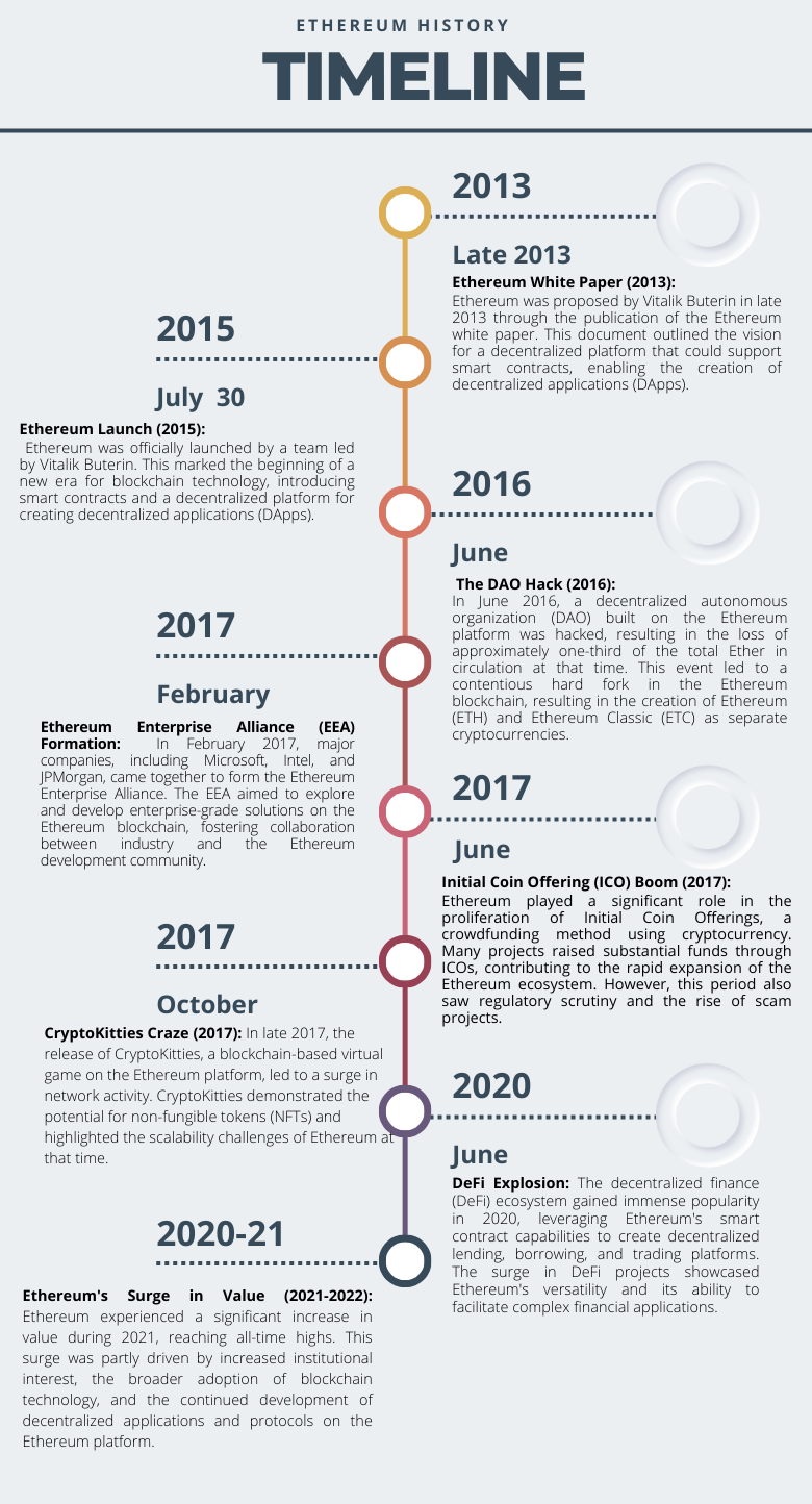
Ethereum is a groundbreaking blockchain platform that emerged in the wake of Bitcoin’s success in 2015. While Bitcoin introduced and popularized the blockchain concept, Ethereum has leveraged this technology more effectively than any other digital currency. Promoters of new projects tend to rely on Ethereum’s tools rather than embark on the lengthy and expensive process of developing a new blockchain. Ethereum was conceived by a young Canadian programmer, Vitalik Buterin, who saw limitations in Bitcoin’s functionality and envisioned a decentralized platform capable of executing smart contracts. Buterin’s idea gained traction in the cryptocurrency community, and he, along with a team of developers, published the Ethereum whitepaper in late 2013. The platform’s official development began in 2014, with a crowdfunding campaign that raised over $18 million in Bitcoin, making it one of the most successful initial coin offerings (ICOs) of its time. Ethereum’s genesis block was mined on July 30, 2015, marking the official launch of the network.
Ethereum’s innovative concept of smart contracts and decentralized applications (DApps) quickly garnered attention within the blockchain and cryptocurrency space. The platform introduced a Turing-complete programming language, enabling developers to create a wide array of decentralized applications. Ethereum’s native cryptocurrency, Ether (ETH), serves as both a digital currency and a utility token within the ecosystem. Over the years, Ethereum has undergone several network upgrades to improve scalability and security, most notably the transition from a proof-of-work (PoW) to a proof-of-stake (PoS) consensus mechanism with the Ethereum 2.0 upgrade. This transition aims to address the network’s scalability issues and reduce its energy consumption, positioning Ethereum as a sustainable and versatile blockchain platform for the future. Today, Ethereum continues to play a pivotal role in the blockchain and decentralized finance (DeFi) space, powering a vast array of projects, including NFT platforms, decentralized exchanges, and decentralized applications that have reshaped the way we think about finance and technology.
Ethereum Logo

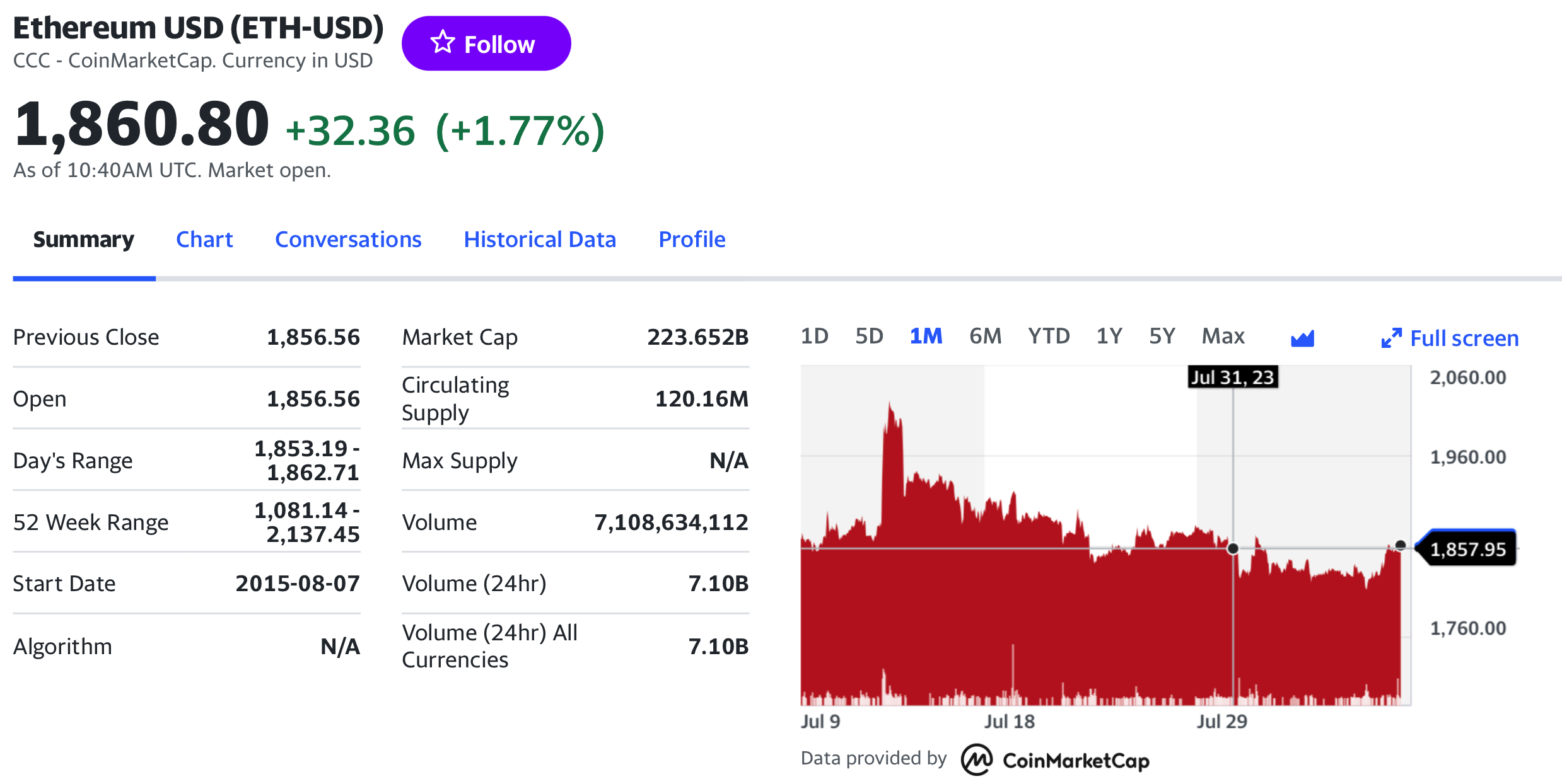
Source: Yahoo! Finance .
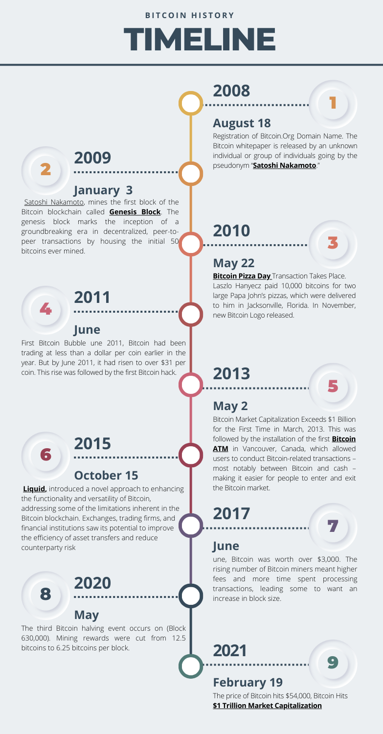
Figure 1. Key Dates in Ethereum History
Source: Yahoo! Finance .
Key Features of Ethereum
Smart Contracts
Ethereum is renowned for its pioneering smart contract functionality. Smart contracts are self-executing agreements with predefined rules and conditions, enabling automated and trustless transactions. This feature has broad applications in various industries, including finance, supply chain management, and legal services.
Decentralization
Ethereum operates on a decentralized network of nodes, making it resistant to censorship and single points of failure. This decentralization ensures the security and integrity of the blockchain, with no single entity having control over the network.
Ether (ETH)
Ethereum’s native cryptocurrency, Ether, serves as both a digital currency and a utility token. It’s used to pay for transaction fees, secure the network through staking in Ethereum 2.0, and as a medium of exchange within the ecosystem.
Interoperability
Ethereum is designed to interact with other blockchains and networks, fostering compatibility and collaboration across the blockchain ecosystem. Projects like Polkadot and Cosmos aim to enhance this interoperability.
EVM (Ethereum Virtual Machine)
The Ethereum Virtual Machine is a runtime environment for executing smart contracts. It’s a critical component that ensures the same execution of smart contracts across all Ethereum nodes, making Ethereum’s ecosystem reliable and consistent.
EIPs (Ethereum Improvement Proposals)
Ethereum has a robust governance model for protocol upgrades and improvements, with EIPs serving as the mechanism for proposing and implementing changes. This allows for community-driven innovation and adaptation.
Use Cases of Ethereum
Decentralized Finance (DeFi)
Ethereum is at the heart of the DeFi movement, offering lending, borrowing, trading, and yield farming services through DApps like Compound, Aave, and Uniswap. DeFi has disrupted traditional finance, providing open and inclusive access to financial services.
Non-Fungible Tokens (NFTs)
Ethereum’s ERC-721 and ERC-1155 token standards have fueled the NFT boom. NFTs enable the ownership and trade of unique digital assets, from art and music to virtual real estate and collectibles, all recorded on the blockchain.
Supply Chain Management
Ethereum’s transparent and tamper-proof ledger is used to track and verify the authenticity and provenance of products. This enhances supply chain efficiency and trust, reducing fraud and counterfeiting.
Gaming and Virtual Worlds
Ethereum is the platform of choice for blockchain-based gaming and virtual reality experiences. DApps like Decentraland and Axie Infinity allow users to trade in-game assets and participate in virtual economies.
Tokenization of Assets
Real-world assets, such as real estate, stocks, and commodities, can be tokenized on the Ethereum blockchain, making them more accessible for investment and trading.
Identity Verification
Ethereum can be used to secure and manage digital identities, enhancing privacy and reducing the risk of identity theft.
Social Impact
Ethereum is leveraged for social impact projects, including humanitarian aid distribution, voting systems, and tracking philanthropic donations, ensuring transparency and accountability.
Content Distribution
Ethereum-based projects are exploring decentralized content platforms, enabling creators to have more control over their intellectual property and revenue.
Ethereum’s versatility and ongoing development make it a crucial platform for a wide range of applications, from financial innovation to social change and beyond, driving the evolution of the blockchain and cryptocurrency space.
Technology and underlying blockchain
Ethereum’s underlying technology is rooted in blockchain, a distributed ledger system known for its security, transparency, and decentralization. Ethereum, like Bitcoin, employs a blockchain to record and verify transactions, but it offers a distinct set of features and capabilities that set it apart. At the core of Ethereum’s technology is the Ethereum Virtual Machine (EVM), a decentralized computing environment that executes smart contracts. Smart contracts are self-executing agreements with predefined rules and conditions that automate processes without the need for intermediaries.
Ethereum uses a consensus mechanism known as Proof of Stake (PoS), which is a significant departure from Bitcoin’s Proof of Work (PoW). PoS allows network participants, known as validators, to create new blocks and secure the network by locking up a certain amount of Ether as collateral. This approach is more energy-efficient and scalable compared to PoW, addressing some of the limitations that Bitcoin faces. Ethereum’s blockchain is a public and permissionless network, meaning that anyone can participate, transact, and develop decentralized applications (DApps) on the platform without needing approval.
The Ethereum ecosystem also employs a variety of token standards, with ERC-20 and ERC-721 being the most well-known. ERC-20 tokens are fungible and often used for cryptocurrencies, while ERC-721 tokens are non-fungible and have powered the explosion of NFTs (Non-Fungible Tokens). These standards have facilitated the creation and interoperability of a vast array of digital assets and DApps on the platform. Ethereum’s robust governance model, through Ethereum Improvement Proposals (EIPs), allows the community to suggest and implement changes, ensuring that the platform remains adaptable and responsive to evolving needs and challenges. Ethereum’s groundbreaking technology and active development community have positioned it as a leader in the blockchain space, with far-reaching implications for industries beyond just cryptocurrencies.
Supply of coins
Ethereum initially used a proof-of-work (PoW) consensus algorithm for coin mining, similar to Bitcoin. The process involved miners solving complex mathematical puzzles to validate transactions and add new blocks to the blockchain. Miners competed to solve these puzzles, and the first one to succeed was rewarded with newly minted Ethereum coins (ETH). This process was resource-intensive and required significant computational power.
However, Ethereum has been undergoing a transition to a proof-of-stake (PoS) consensus mechanism as part of its Ethereum 2.0 upgrade. The PoS model doesn’t rely on miners solving computational puzzles but instead relies on validators who lock up a certain amount of cryptocurrency as collateral to propose and validate new blocks. Validators are chosen to create new blocks based on the amount of cryptocurrency they hold and are willing to “stake” as collateral.
This transition to PoS is occurring in multiple phases. The Beacon Chain, which is the PoS blockchain that runs parallel to the existing PoW chain, was launched in December 2020. The full transition to Ethereum 2.0, including the complete shift to PoS, is expected to occur in multiple subsequent phases.
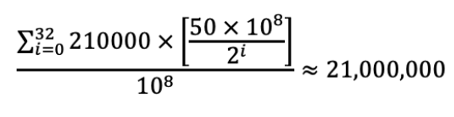
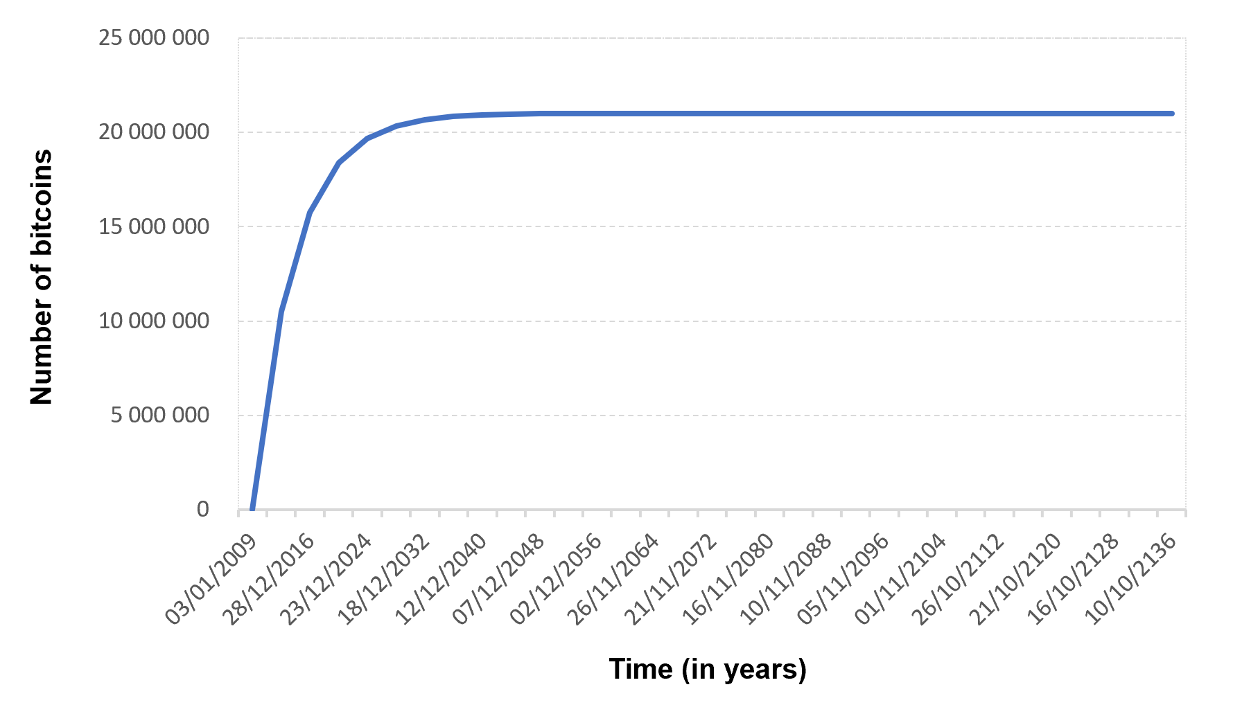
As of Q1 2023, there are approximately 121,826,163.06 Ethereum (ETH) coins in circulation, a key distinction from Bitcoin, which has a capped supply of 21 million. Ethereum, created by Vitalik Buterin, was designed without a specific supply limit, allowing for an unlimited number of coins if mining continues. Despite this, there is a cap of 18 million ETH coins that can be mined annually, equating to around 2 ETH per block. Ethereum Classic (ETC), a separate blockchain resulting from a community dispute, also exists with 135.3 billion coins. The Ethereum blockchain’s size was 175 GB in 2021, considerably smaller than Bitcoin’s 412 GB. Approximately 5750 Ethereum blocks are mined daily, with mining difficulty increasing and around 2,151 active nodes globally, primarily in the USA. Ethereum’s potential to become deflationary is acknowledged, contingent on mining costs exceeding rewards, as stated in a GitHub disclaimer.
Figure 2. Number of Ethereum Transaction per Day
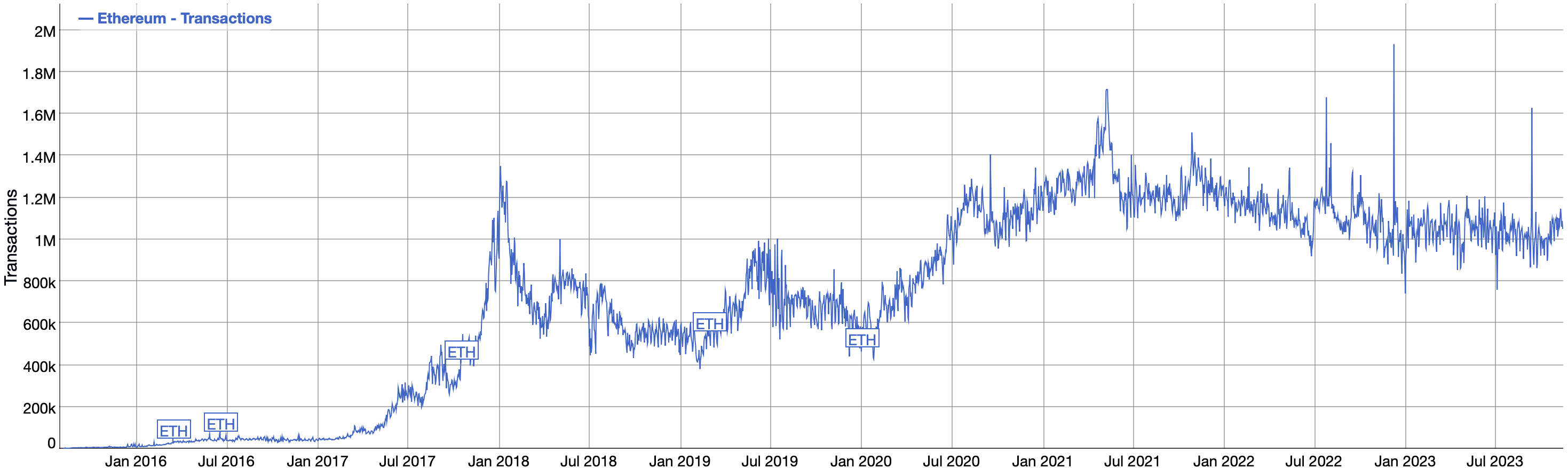
Source: BitInfoCharts (Ethereum Transactions historical chart).
Historical data for Ethereum
How to get the data?
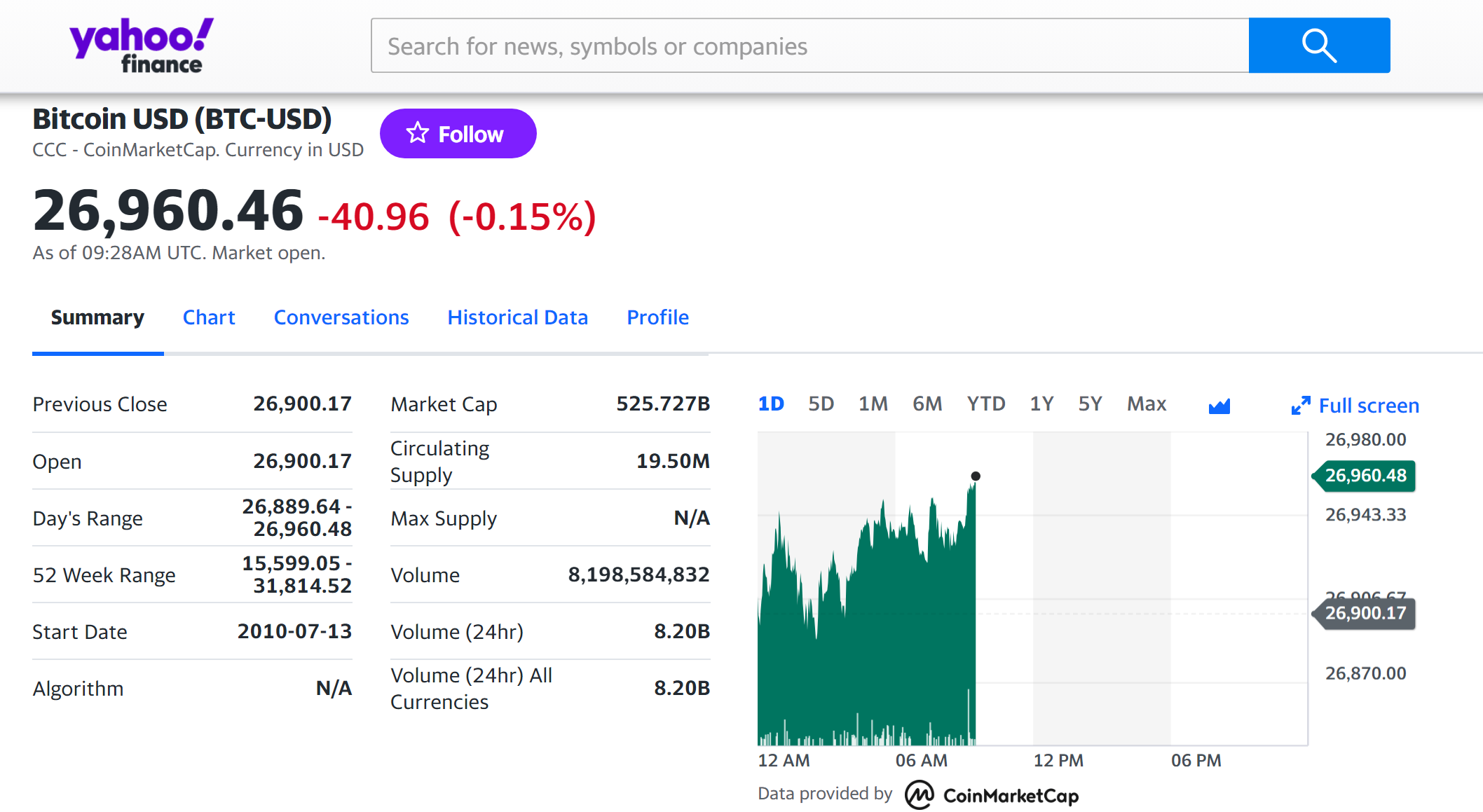
The Ethereum is the most popular cryptocurrency on the market, and historical data for the Ethereum such as prices and volume traded can be easily downloaded from the internet sources such as Yahoo! Finance, Blockchain.com & CoinMarketCap. For example, you can download data for Ethereum on Yahoo! Finance (the Yahoo! code for Ethereum is ETH-USD).
Figure 4. Ethereum data
Source: Yahoo! Finance.
Historical data for the Ethereum market prices
Historical data on the price of Ethereum holds paramount significance in understanding the cryptocurrency’s market trends, investor behavior, and overall performance over time. Analyzing historical price data allows investors, analysts, and researchers to identify patterns, cycles, and potential indicators that may influence future price movements. It provides valuable insights into market sentiment, periods of volatility, and the impact of significant events or developments within the Ethereum ecosystem. Traders use historical data to formulate strategies, assess risk, and make informed decisions. Furthermore, the data aids in evaluating the success of protocol upgrades, regulatory changes, and shifts in broader economic conditions, offering a comprehensive view of Ethereum’s evolution. The historical price data of Ethereum serves as a crucial tool for market participants seeking to navigate the dynamic and sometimes unpredictable nature of the cryptocurrency market.
With the number of coins in circulation, the information on the price of coins for a given currency is also important to compute Ethereum’s market capitalization.
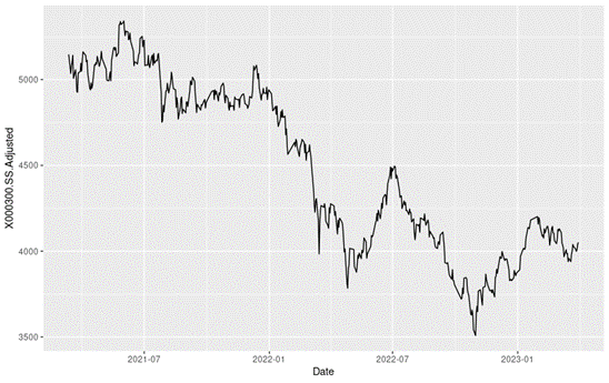
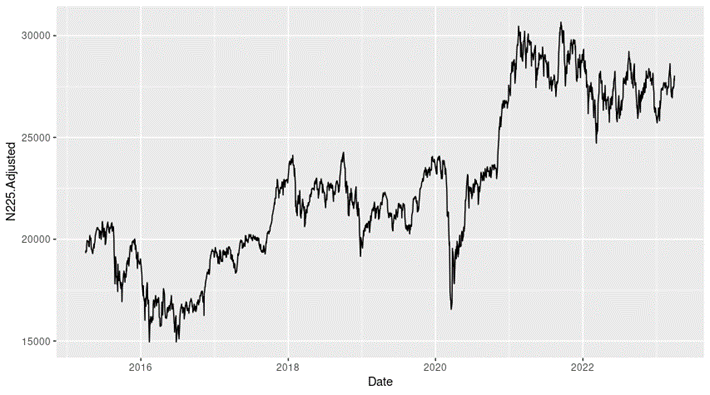
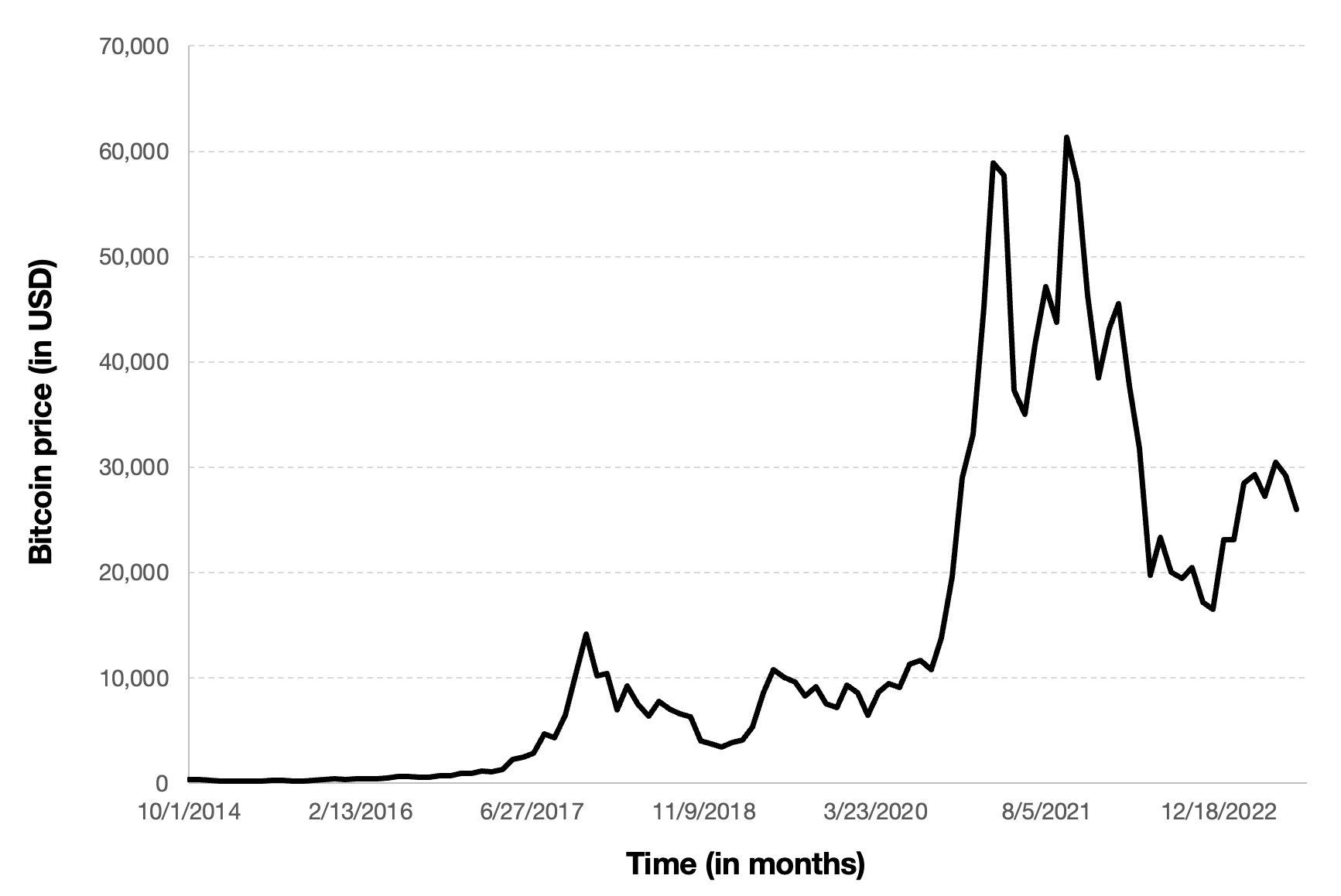
Figure 5 below represents the evolution of the price of Ethereum in US dollar over the period Nov 2017 – Dec 2023. The price corresponds to the “closing” price (observed at 10:00 PM CET at the end of the month).
Figure 5. Evolution of the Ethereum price
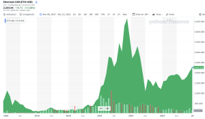
Source: Yahoo! Finance.
R program
The R program below written by Shengyu ZHENG allows you to download the data from Yahoo! Finance website and to compute summary statistics and risk measures about the Ethereum.

Data file
The R program that you can download above allows you to download the data for the Ethereum from the Yahoo! Finance website. The database starts on December, 2017.
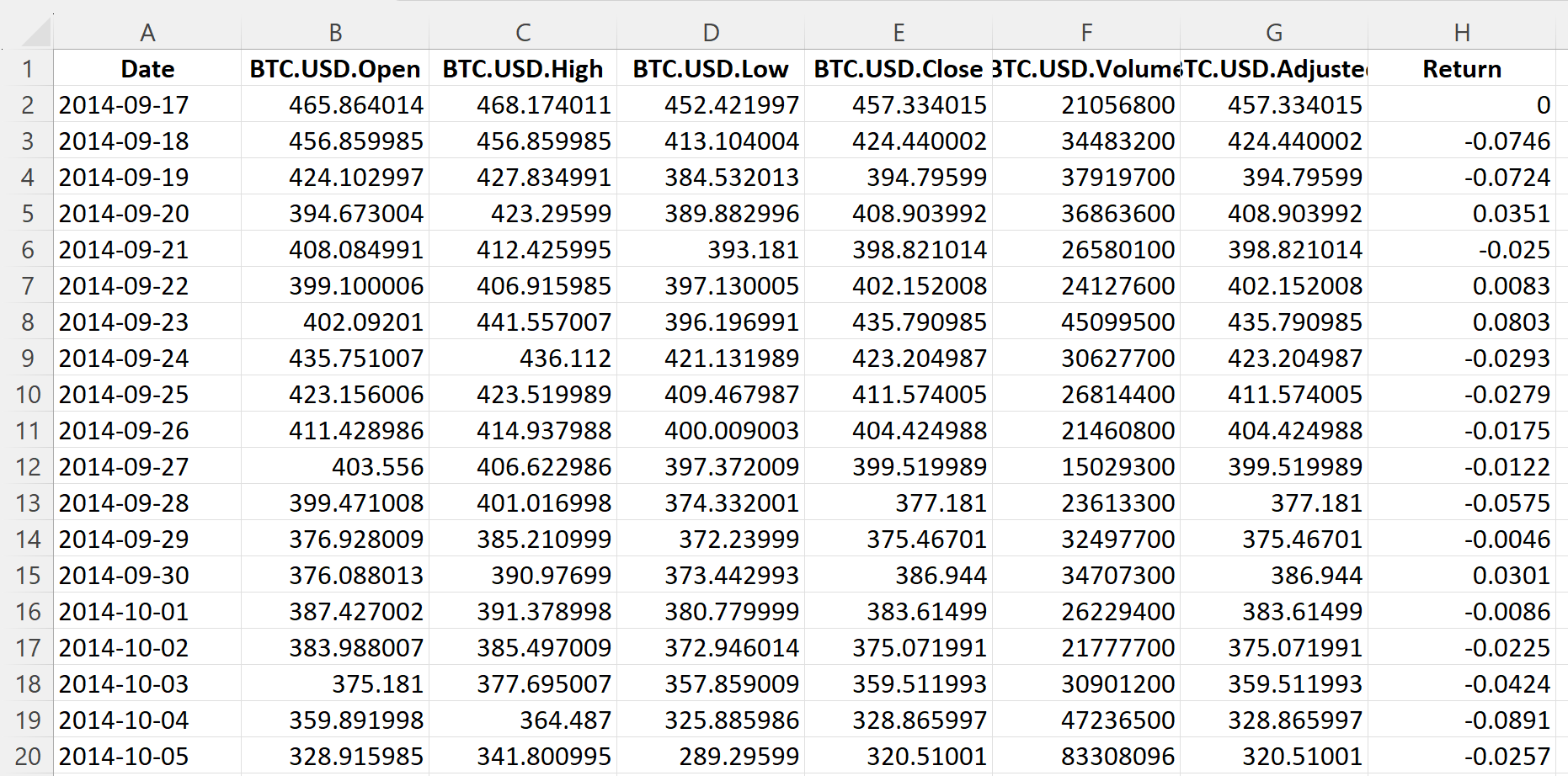
Table 3 below represents the top of the data file for the Ethereum downloaded from the Yahoo! Finance website with the R program.
Table 3. Top of the data file for the Ethereum.
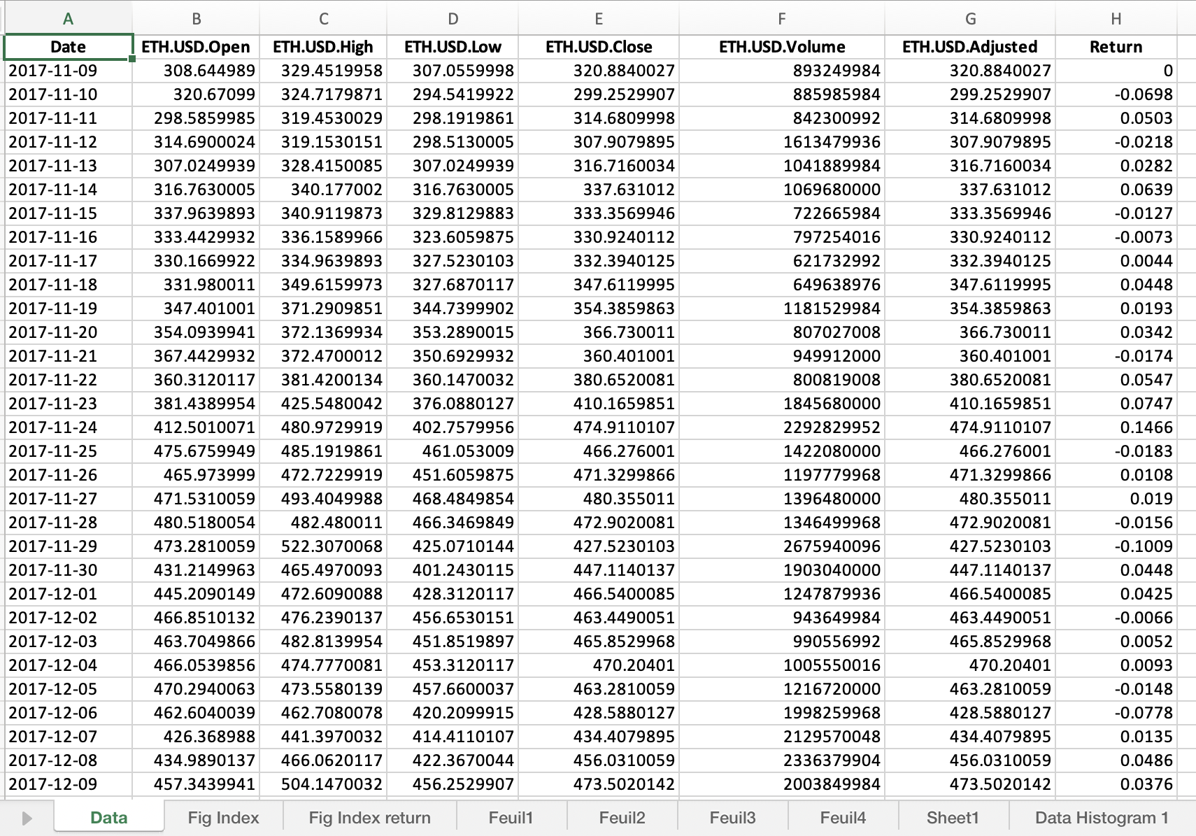
Source: computation by the author (data: Yahoo! Finance website).
Python code
You can download the Python code used to download the data from Yahoo! Finance.

Python script to download Ethereum historical data and save it to an Excel sheet::
import yfinance as yf
import pandas as pd
# Define the ticker symbol for Ethereum
eth_ticker = “ETH-USD”
# Define the date range for historical data
start_date = “2020-01-01”
end_date = “2022-01-01”
# Download historical data using yfinance
eth_data = yf.download(eth_ticker, start=start_date, end=end_date)
# Create a Pandas DataFrame from the downloaded data
eth_df = pd.DataFrame(eth_data)
# Define the Excel file path
excel_file_path = “ethereum_historical_data.xlsx”
# Save the data to an Excel sheet
eth_df.to_excel(excel_file_path, sheet_name=”ETH Historical Data”)
print(f”Data saved to {excel_file_path}”)
# Make sure you have the required libraries installed and adjust the “start_date” and “end_date” variables to the desired date range for the historical data you want to download.
Evolution of the Ethereum
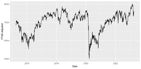
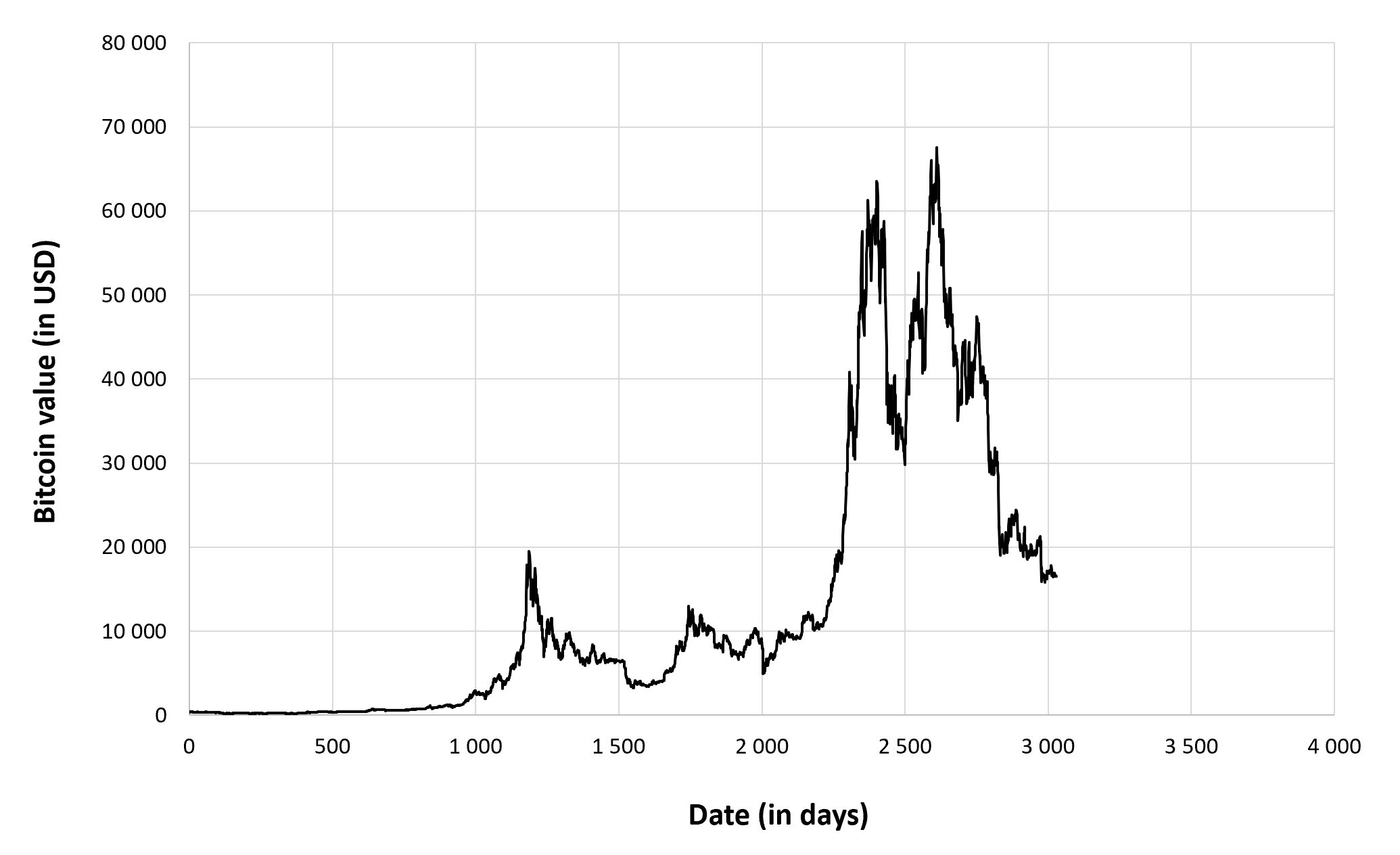
Figure 6 below gives the evolution of the Ethereum on a daily basis.
Source: computation by the author (data: Yahoo! Finance website).
Figure 6. Evolution of the Ethereum.
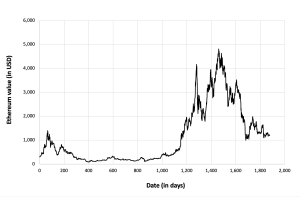
Source: computation by the author (data: Yahoo! Finance website).
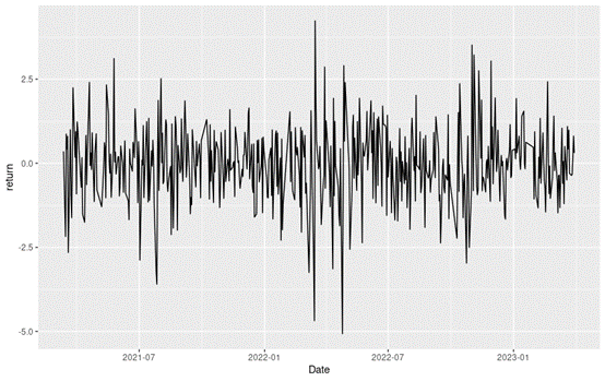
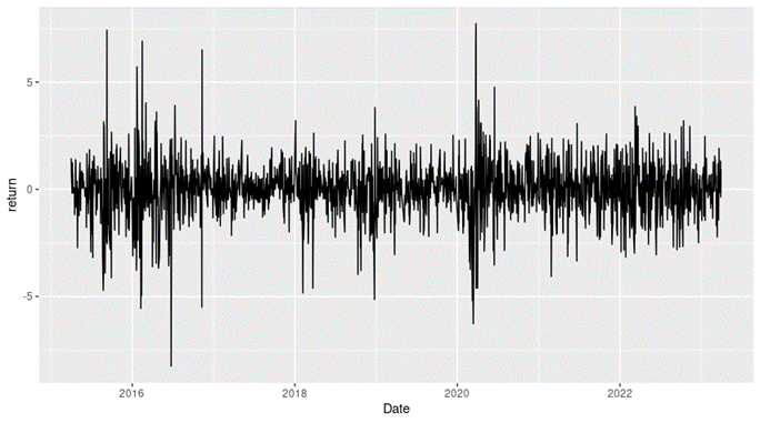
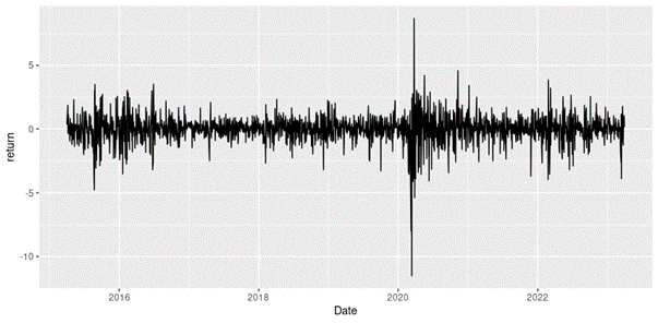
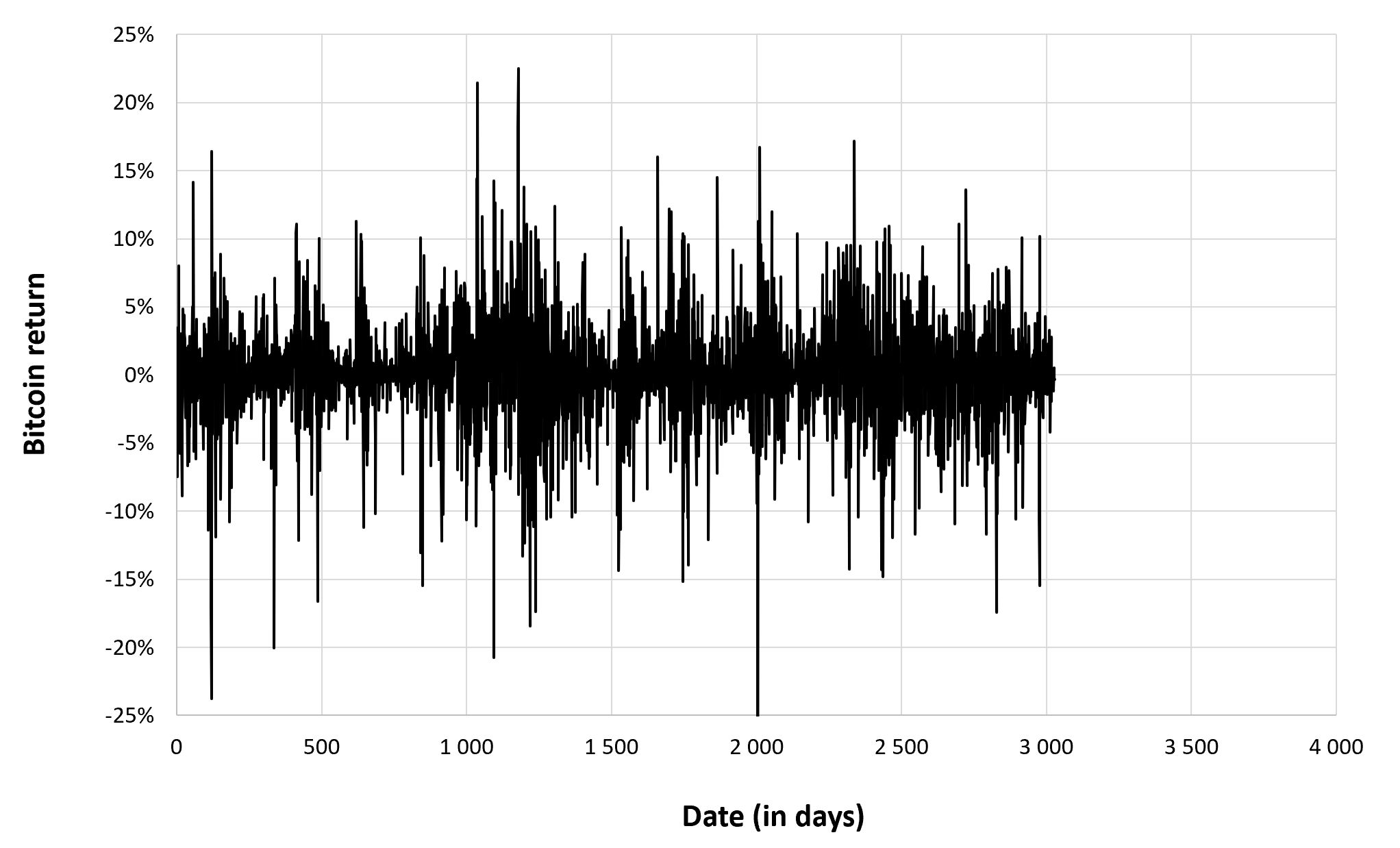
Figure 2 below gives the evolution of the Ethereum returns from November 09, 2017 to December 31, 2022 on a daily basis.
Figure 7. Evolution of the Ethereum returns.
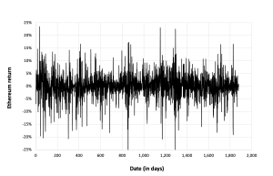
Source: computation by the author (data: Yahoo! Finance website).
Summary statistics for the Ethereum
The R program that you can download above also allows you to compute summary statistics about the returns of the Ethereum.
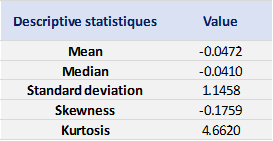
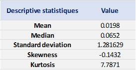
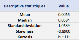
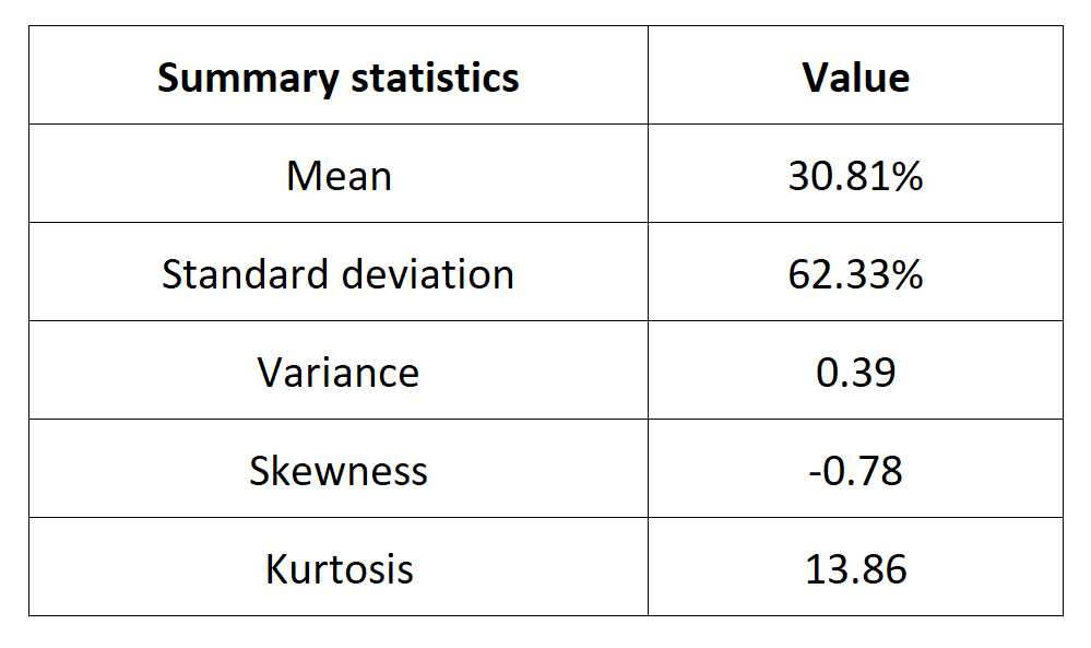
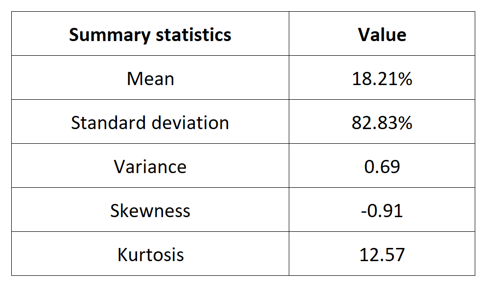
Table 4 below presents the following summary statistics estimated for the Ethereum:
- The mean
- The standard deviation (the squared root of the variance)
- The skewness
- The kurtosis.
The mean, the standard deviation / variance, the skewness, and the kurtosis refer to the first, second, third and fourth moments of statistical distribution of returns respectively.
Table 4. Summary statistics for the Ethereum.
Source: computation by the author (data: Yahoo! Finance website).
Statistical distribution of the Ethereum returns
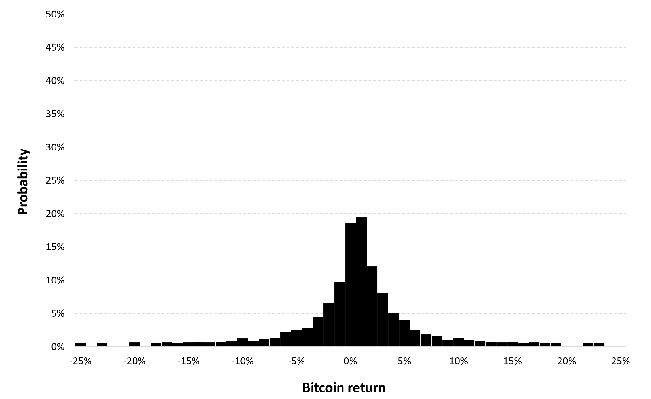
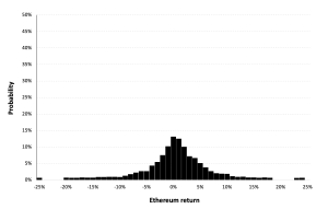
Historical distribution
Figure 8 represents the historical distribution of the Ethereum daily returns for the period from November 09, 2017 to December 31, 2022.
Figure 8. Historical Ethereum distribution of the returns.
Source: computation by the author (data: Yahoo! Finance website).
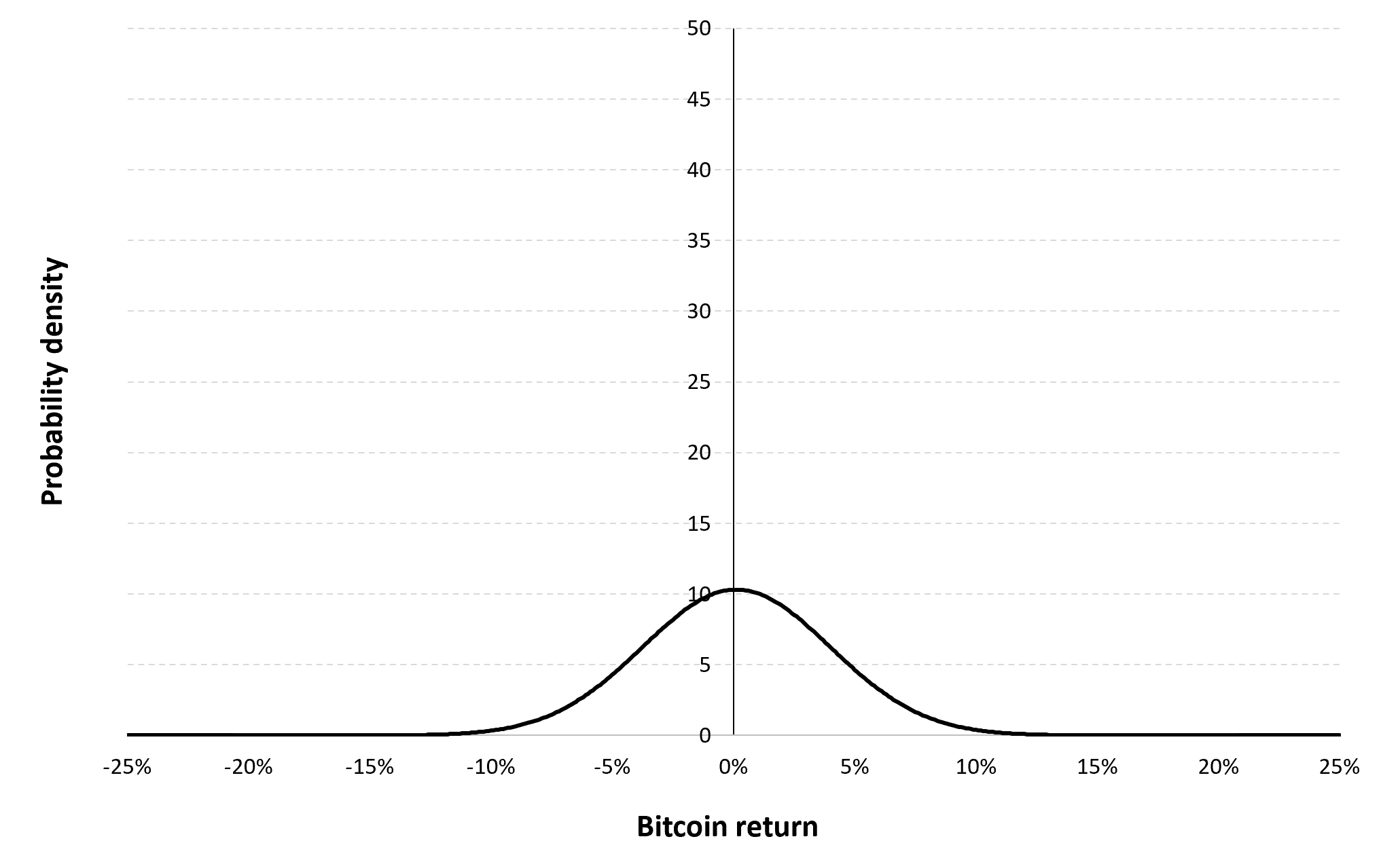
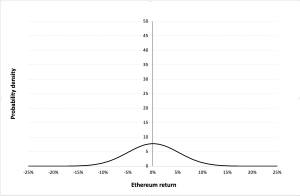
Gaussian distribution
The Gaussian distribution (also called the normal distribution) is a parametric distribution with two parameters: the mean and the standard deviation of returns. We estimated these two parameters over the period from November 09, 2017 to December 31, 2022. The annualized mean of daily returns is equal to 30.81% and the annualized standard deviation of daily returns is equal to 62.33%.
Figure 9 below represents the Gaussian distribution of the Ethereum daily returns with parameters estimated over the period from November 09, 2017 to December 31, 2022.
Figure 9. Gaussian distribution of the Ethereum returns.
Source: computation by the author (data: Yahoo! Finance website).
Risk measures of the Ethereum returns
The R program that you can download above also allows you to compute risk measures about the returns of the Ethereum.
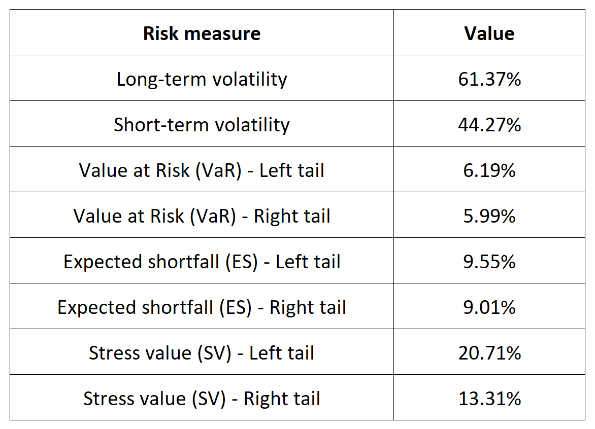
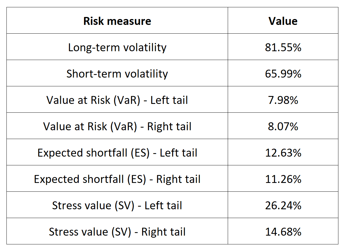
Table 5 below presents the following risk measures estimated for the Ethereum:
- The long-term volatility (the unconditional standard deviation estimated over the entire period)
- The short-term volatility (the standard deviation estimated over the last three months)
- The Value at Risk (VaR) for the left tail (the 5% quantile of the historical distribution)
- The Value at Risk (VaR) for the right tail (the 95% quantile of the historical distribution)
- The Expected Shortfall (ES) for the left tail (the average loss over the 5% quantile of the historical distribution)
- The Expected Shortfall (ES) for the right tail (the average loss over the 95% quantile of the historical distribution)
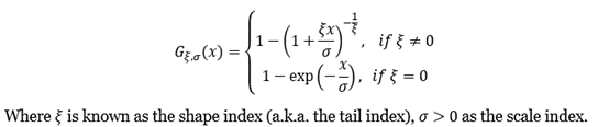
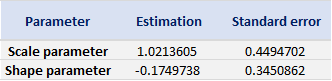
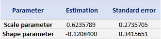
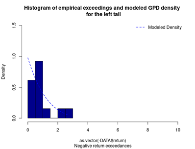
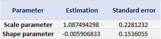
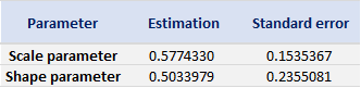
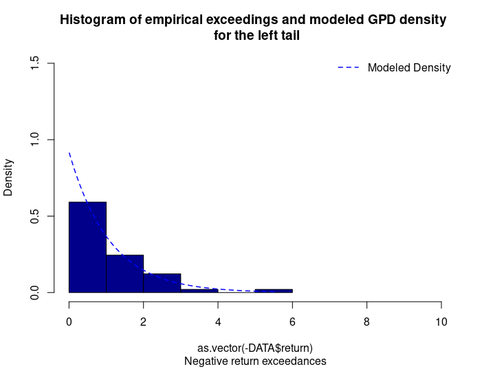
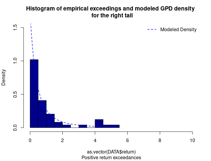
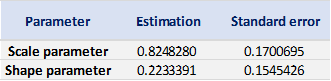
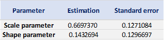
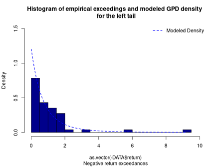
- The Stress Value (SV) for the left tail (the 1% quantile of the tail distribution estimated with a Generalized Pareto distribution)
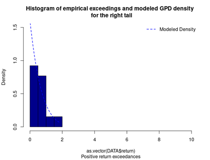
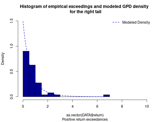
- The Stress Value (SV) for the right tail (the 99% quantile of the tail distribution estimated with a Generalized Pareto distribution)
Table 5. Risk measures for the Ethereum.
Source: computation by the author (data: Yahoo! Finance website).
The volatility is a global measure of risk as it considers all the returns. The Value at Risk (VaR), Expected Shortfall (ES) and Stress Value (SV) are local measures of risk as they focus on the tails of the distribution. The study of the left tail is relevant for an investor holding a long position in the Ethereum while the study of the right tail is relevant for an investor holding a short position in the Ethereum.
Why should I be interested in this post?
Ethereum, the pioneering blockchain platform, is an essential topic for management students due to its potential to transform industries, create innovative business opportunities, and disrupt traditional financial systems. Understanding Ethereum’s smart contracts, DeFi ecosystem, NFT market, and global impact can provide students with a competitive edge in a rapidly evolving business landscape, enabling them to navigate emerging trends, make informed investment decisions, and explore entrepreneurship in the digital economy.
Related posts on the SimTrade blog
About cryptocurrencies
▶ Snehasish CHINARA Bitcoin: the mother of all cryptocurrencies
▶ Snehasish CHINARA How to get crypto data
▶ Alexandre VERLET Cryptocurrencies
▶ Youssef EL QAMCAOUI Decentralised Financing
▶ Hugo MEYER The regulation of cryptocurrencies: what are we talking about?
About statistics
▶ Shengyu ZHENG Moments de la distribution
▶ Shengyu ZHENG Mesures de risques
▶ Jayati WALIA Returns
Useful resources
Academic research about risk
Longin F. (2000) From VaR to stress testing: the extreme value approach Journal of Banking and Finance, N°24, pp 1097-1130.
Longin F. (2016) Extreme events in finance: a handbook of extreme value theory and its applications Wiley Editions.
Data
Yahoo! Finance
Yahoo! Finance Historical data for Ethereum
CoinMarketCap Historical data for Ethereum
About the author
The article was written in December 2023 by Snehasish CHINARA (ESSEC Business School, Grande Ecole Program – Master in Management, 2022-2024).