In this article, Martin VAN DER BORGHT (ESSEC Business School, Master in Finance, 2022-2024) explains the key financial concept of market efficiency.
What is Market Efficiency?
Market efficiency is an economic concept that states that financial markets are efficient when all relevant information is accurately reflected in the prices of assets. This means that the prices of assts reflect all available information and that no one can consistently outperform the market by trading on the basis of this information. Market efficiency is often measured by the degree to which prices accurately reflect all available information.
The efficient market hypothesis (EMH) states that markets are efficient and that it is impossible to consistently outperform the market by utilizing available information. This means that any attempt to do so will be futile and that all investors can expect to earn the same expected return over time. The EMH is based on the idea that prices are quickly and accurately adjusted to reflect new information, which means that no one can consistently make money by trading on the basis of this information.
Types of Market Efficiency
Following Fama’s academic works, there are three different types of market efficiency: weak, semi-strong, and strong.
Weak form of market efficiency
The weak form of market efficiency states that asset prices reflect all information from past prices and trading volumes. This implies that technical analysis, which is the analysis of past price and volume data to predict future prices, is not an effective way to outperform the market.
Semi-strong form of market efficiency
The semi-strong form of market efficiency states that asset prices reflect all publicly available information, including financial statements, research reports, and news. This implies that fundamental analysis, which is the analysis of a company’s financial statements and other publicly available information to predict future prices, is also not an effective way to outperform the market.
Strong form of market efficiency
Finally, the strong form of market efficiency states that prices reflect all available information, including private information. This means that even insider trading, which is the use of private information to make profitable trades, is not an effective way to outperform the market.
The Grossman-Stiglitz paradox
If financial markets are informationally efficient in the sense they incorporate all relevant information available, then considering this information is useless when making investment decisions in the sense that this information cannot be used to beat the market on the long term. We may wonder how this information can be incorporate in the market prices if no market participants look at information. This is the Grossman-Stiglitz paradox.
Real-Life Examples of Market Efficiency
The efficient market hypothesis has been extensively studied and there are numerous examples of market efficiency in action.
NASDAQ IXIC 1994 – 2005
One of the most famous examples is the dot-com bubble of the late 1990s. During this time, the prices of tech stocks skyrocketed to levels that were far higher than their fundamental values. This irrational exuberance was quickly corrected as the prices of these stocks were quickly adjusted to reflect the true value of the companies.
NASDAQ IXIC Index, 1994-2005
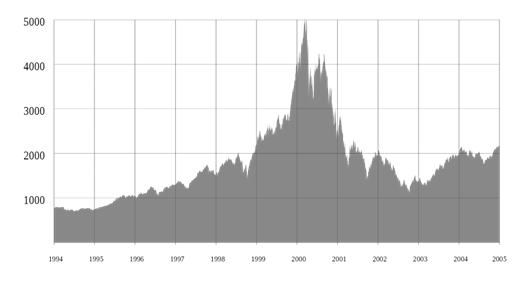
Source: Wikimedia.
The figure “NASDAQ IXIC Index, 1994-2005” shows the Nasdaq Composite Index (IXIC) from 1994 to 2005. During this time period, the IXIC experienced an incredible surge in value, peaking in 2000 before its subsequent decline. This was part of the so-called “dot-com bubble” of the late 1990s and early 2000s, when investors were optimistic about the potential for internet-based companies to revolutionize the global economy.
The IXIC rose from around 400 in 1994 to a record high of almost 5000 in March 2000. This was largely due to the rapid growth of tech companies such as Amazon and eBay, which attracted huge amounts of investment from venture capitalists. These investments drove up stock prices and created a huge market for initial public offerings (IPOs).
However, this rapid growth was not sustainable, and by the end of 2002 the IXIC had fallen back to around 1300. This was partly due to the bursting of the dot-com bubble, as investors began to realize that many of the companies they had invested in were unprofitable and overvalued. Many of these companies went bankrupt, leading to large losses for their investors.
Overall, the figure “Indice IXIC du NASDAQ, 1994-2005” illustrates the boom and bust cycle of the dot-com bubble, with investors experiencing both incredible gains and huge losses during this period. It serves as a stark reminder of the risks associated with investing in tech stocks. During this period, investors were eager to pour money into internet-based companies in the hopes of achieving huge returns. However, many of these companies were unprofitable, and their stock prices eventually plummeted as investors realized their mistake. This led to large losses for investors, and the bursting of the dot-com bubble.
In addition, this period serves as a reminder of the importance of proper risk management when it comes to investing. While it can be tempting to chase high returns, it is important to remember that investments can go up as well as down. By diversifying your portfolio and taking a long-term approach, you can reduce your risk profile and maximize your chances of achieving successful returns.
U.S. Subprime lending expanded dramatically 2004–2006.
Another example of market efficiency is the global financial crisis of 2008. During this time, the prices of many securities dropped dramatically as the market quickly priced in the risks associated with rising defaults and falling asset values. The market was able to quickly adjust to the new information and the prices of securities were quickly adjusted to reflect the new reality.
U.S. Subprime Lending Expanded Significantly 2004-2006
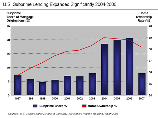
Source: US Census Bureau.
The figure “U.S. Subprime lending expanded dramatically 2004–2006” illustrates the extent to which subprime mortgage lending in the United States increased during this period. It shows a dramatic rise in the number of subprime mortgages issued from 2004 to 2006. In 2004, less than $500 billion worth of mortgages were issued that were either subprime or Alt-A loans. By 2006, that figure had risen to over $1 trillion, an increase of more than 100%.
This increase in the number of subprime mortgages being issued was largely driven by lenders taking advantage of relaxed standards and government policies that encouraged home ownership. Lenders began offering mortgages with lower down payments, looser credit checks, and higher loan-to-value ratios. This allowed more people to qualify for mortgages, even if they had poor credit or limited income.
At the same time, low interest rates and a strong economy made it easier for people to take on these loans and still be able to make their payments. As a result, many people took out larger mortgages than they could actually afford, leading to an unsustainable increase in housing prices and eventually a housing bubble.
When the bubble burst, millions of people found themselves unable to make their mortgage payments, and the global financial crisis followed. The dramatic increase in subprime lending seen in this figure is one of the primary factors that led to the 2008 financial crisis and is an illustration of how easily irresponsible lending can lead to devastating consequences.
Impact of FTX crash on FTT
Finally, the recent rise (and fall) of the cryptocurrency market is another example of market efficiency. The prices of cryptocurrencies have been highly volatile and have been quickly adjusted to reflect new information. This is due to the fact that the market is highly efficient and is able to quickly adjust to new information.
Price and Volume of FTT
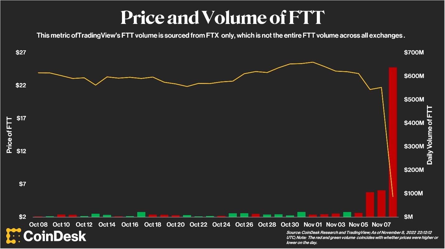
Source: CoinDesk.
FTT price and volume is a chart that shows the impact of the FTX exchange crash on the FTT token price and trading volume. The chart reflects the dramatic drop in FTT’s price and the extreme increase in trading volume that occurred in the days leading up to and following the crash. The FTT price began to decline rapidly several days before the crash, dropping from around $3.60 to around $2.20 in the hours leading up to the crash. Following the crash, the price of FTT fell even further, reaching a low of just under $1.50. This sharp drop can be seen clearly in the chart, which shows the steep downward trajectory of FTT’s price.
The chart also reveals an increase in trading volume prior to and following the crash. This is likely due to traders attempting to buy low and sell high in response to the crash. The trading volume increased dramatically, reaching a peak of almost 20 million FTT tokens traded within 24 hours of the crash. This is significantly higher than the usual daily trading volume of around 1 million FTT tokens.
Overall, this chart provides a clear visual representation of the dramatic impact that the FTX exchange crash had on the FTT token price and trading volume. It serves as a reminder of how quickly markets can move and how volatile they can be, even in seemingly stable assets like cryptocurrencies.
Today, the FTT token price has recovered somewhat since the crash, and currently stands at around $2.50. However, this is still significantly lower than it was prior to the crash. The trading volume of FTT is also much higher than it was before the crash, averaging around 10 million tokens traded per day. This suggests that investors are still wary of the FTT token, and that the market remains volatile.
Conclusion
Market efficiency is an important concept in economics and finance and is based on the idea that prices accurately reflect all available information. There are three types of market efficiency, weak, semi-strong, and strong, and numerous examples of market efficiency in action, such as the dot-com bubble, the global financial crisis, and the recent rise of the cryptocurrency market. As such, it is clear that markets are generally efficient and that it is difficult, if not impossible, to consistently outperform the market.
Related posts on the SimTrade blog
▶ All posts related to market efficiency
▶ William ANTHONY Peloton’s uphill battle with the world’s return to order
▶ Aamey MEHTA Market efficiency: the case study of Yes bank in India
▶ Aastha DAS Why is Apple’s new iPhone 14 release line failing in the first few months?
Useful resources
SimTrade course Market information
Academic research
Fama E. (1970) Efficient Capital Markets: A Review of Theory and Empirical Work, Journal of Finance, 25, 383-417.
Fama E. (1991) Efficient Capital Markets: II Journal of Finance, 46, 1575-617.
Grossman S.J. and J.E. Stiglitz (1980) On the Impossibility of Informationally Efficient Markets The American Economic Review, 70, 393-408.
Chicago Booth Review (30/06/2016) Are markets efficient? Debate between Eugene Fama and Richard Thaler (YouTube video)
Business resources
CoinDesk These Four Key Charts Shed Light on the FTX Exchange’s Spectacular Collapse
Bloomberg Crypto Prices Fall Most in Two Weeks Amid FTT and Macro Risks
About the author
The article was written in January 2023 by Martin VAN DER BORGHT (ESSEC Business School, Master in Finance, 2022-2024).


 Source: computation by the author (data: Refinitiv Eikon).
 Source: computation by the author (Data: Refinitiv Eikon).
 Source: computation by the author (Data: Bloomberg)
 Source: computation by the author. (Data: Reuters Eikon)