

In this article, Youssef LOURAOUI (ESSEC Business School, Global Bachelor of Business Administration, 2017-2021) presents the origin of factor investing. A factor is defined as a persistent driver that helps explain assets’ long-term risk and return properties across asset classes.
This article is structured as follows: we begin by presenting Markowitz’s Modern Portfolio Theory (MPT) as the origin of factor investing (market factor). We then explain the Fama-French three-factor models, which is an extension of the CAPM single factor model (market factor). Furthermore, we explain also the Carhart four-factor model and the Fama-French five-factor model that aimed to capture additional factors to the market factor.
Markowitz’s Modern Portfolio Theory: Origin of the factor investing
Factor investing can be retraced to the work of Harry Markowitz in the early 1950s. The most important aspect of Markowitz’s approach was his fundamental finding that an asset’s risk and return should not be evaluated on its own, but rather on how it contributes to the entire risk and return of a portfolio. His dissertation, titled “Portfolio Selection”, was published in The Journal of Finance (1952). Nearly thirty years later, Markowitz shared the Nobel Prize for economics and corporate finance for his MPT contributions to both disciplines. The holy grail of Markowitz’s work is based on his calculation of the variance of a two-asset portfolio computed as follows:
![]()
Where:
- w and (1-w) represents asset weights of assets A and B
- σ2 represents the variance of the assets and portfolio
- cov(rA,rB) represents the covariance of assets A and B.
Capital Asset Pricing Model (CAPM)
William Sharpe, John Lintner, and Jan Mossin separately developed another key capital markets theory as a result of Markowitz’s previous works : the Capital Asset Pricing Model (CAPM). The CAPM was a huge evolutionary step forward in capital market equilibrium theory, since it enabled investors to appropriately value assets in terms of systematic risk, defined as the market risk which cannot be neutralized by the effect of diversification. In his derivation of the CAPM, Sharpe, Mossin and Litner made significant contributions to the concepts of the Efficient Frontier and Capital Market Line. Sharpe, Litner and Mossin seminal contributions would later earn him the Nobel Prize in Economics. The CAPM is based on a set of market structure and investor hypotheses:
- There are no intermediaries
- There are no limits (short selling is possible)
- Supply and demand are in balance
- There are no transaction costs
- An investor’s portfolio value is maximized by maximizing the mean associated with projected returns while reducing risk variance
- Investors have simultaneous access to information in order to implement their investment plans
- Investors are seen as “rational” and “risk averse”.
Under this framework, the expected return of a given asset is related to its risk measured by the beta:
![]()
Where :
- E(r) represents the expected return of the asset
- rf the risk-free rate
- β a measure of the risk of the asset
- E(rm) the expected return of the market
- E[rm– rf]represents the market risk premium.
In this model, the beta (β) parameter is a key parameter and is defined as:
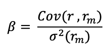
Where:
- Cov(r, rm) represents the covariance of the asset with the market
- σ2(rm) is the variance of market return.
The beta is a measure of how sensitive an asset is to market swings. This risk indicator aids investors in predicting the fluctuations of their asset in relation to the wider market. It compares the volatility of an asset to the systematic risk that exists in the market. The beta is a statistical term that denotes the slope of a line formed by a regression of data points comparing stock returns to market returns. It aids investors in understanding how the asset moves in relation to the market. According to Fama and French (2004), there are two ways to interpret the beta employed in the CAPM:
- According to the CAPM formula, beta may be thought in mathematical terms as the slope of the regression between the asset return and the market return. Thus, beta quantifies the asset sensitivity to changes in the market return;
- According to the beta formula, it may be understood as the risk that each dollar invested in an asset adds to the market portfolio. This is an economic explanation based on the observation that the market portfolio’s risk (measured by 〖σ(r_m)〗^2) is a weighted average of the covariance risks associated with the assets in the market portfolio, making beta a measure of the covariance risk associated with an asset in comparison to the variance of the market return.
Additionally, the CAPM makes a distinction between two forms of risk: systematic and specific risk. Systematic risk refers to the risk posed by the market’s basic structure, its participants, and any and all non-diversifiable elements such as monetary policy, political events, and natural disasters. By contrast, specific risk refers to the risk inherent in a particular asset and so is diversifiable. As a result, the CAPM solely captures systematic risk via the beta measure, with the market’s beta equal to one, lower-risk assets having a beta less than one, and higher-risk assets having a beta larger than one.
Finally, the CAPM’s central message is that when investors invest in a particular security/portfolio, they are rewarded twice: once via the time value of money impact (reflected in the risk-free component of the CAPM equation) and once via the effect of taking on more risk. However, the CAPM is not an empirically sound model, owing to an unnecessarily simplified set of assumptions and problems in establishing validating tests at the model’s first introduction (Fama and French, 2004). Thus, throughout time, the CAPM has been revised and modified to address not just its inadequacies but also to keep pace with financial and economic changes. Sharpe (1990), in his evaluation of the CAPM, cites various examples of revisions to his basic model proposed by other economists and financial experts.
The Fama-French three-factor model
Eugene Fama and Kenneth French created the Fama-French Three-Factor model in 1993 in response to the CAPM’s inadequacy. It contends that, in addition to the market risk component introduced by the CAPM, two more factors affect the returns on securities and portfolios: market capitalization (referred to as the “size” factor) and the book-to-market ratio (referred to as the “value” factor). According to Fama and French, the primary rationale for include these characteristics is because both size and book-to-market (BtM) ratios are related to the economic fundamentals of the business issuing the securities (Fama and French, 1993).
They continue by stating that:
- Earnings and book-to-market ratios are inversely associated, with companies with low book-to-market ratios consistently reporting better earnings than those with high book-to-market ratios
- Due to a similar risk component, size and average returns are inversely associated. This is based on their observation of the trajectory of small business profits in the 1980s: they suggest that small enterprises experience longer durations of earnings depression than larger enterprises in the event of a recession in the economy in which they operate. Additionally, they noted that smaller enterprises did not contribute to the economic expansion in the mid- and late-1980s following the 1982 recession
- Profitability is connected to both size and BtM, and is a common risk factor that emphasizes and explains the positive association between BtM ratios and average returns. As thus, the return on a security/portfolio becomes:

Where :
- E(𝑟) is the expected return of the asset/portfolio
- 𝑟𝑓 is the risk-free rate
- 𝛽 is the measure of the market risk of the asset
- 𝐸(𝑟𝑀) is the expected return of the market
- 𝛽𝑆 is the measure of the risk related to the size of the asset
- 𝛽𝑉 is the measure of the risk related to the value of the security/portfolio
- 𝑆𝑀𝐵 (which stands for “Small Minus Big”) measures the difference in expected returns between small and big firms (in terms of market capitalization)
- 𝐻𝑀𝐿 (which stands for “High Minus Low”) measures the difference in expected returns between value stocks and growth stock
- 𝛼 is a regression intercept
- 𝜖 is a measure of regression error
Both SMB and HML are derived using historical data as well as a mixture of portfolios focused on size and value. Professor French publishes these values on a regular basis on his personal website. Meanwhile, the betas for both the size and value components are derived using linear regression and might be positive or negative. However, the Fama-French three-factor model is not without flaws. Griffin (2002) highlights a significant flaw in the model when he claims that the Fama-French components of value and size are more accurate at explaining return differences when applied locally rather than internationally. As a result, each of the components should be addressed on a nation-by-country basis (as professor French now does on his website, where he specifies the SMB and HML factors for each nation, such as the United Kingdom, France, and so on). While the Fama-French model has gone further than the CAPM in terms of breaking down security returns, it remains an incomplete model with spatially confined interpretation of its additional variables. Efforts have been made over the years to complete this model, with Fama and French adding two more variables in 2015, profitability and investment strategy, and other scholars, like as Carhart (1997), adding a fourth feature, momentum, to the original Three-Factor model.
The Carhart four-factor model
Carhart (1997) extended the Fama-French three-factor model (1993) by adding a fourth factor: momentum. Momentum is defined as the observable tendency for prices to continue climbing or declining following an initial increase or decline. By definition, momentum is an anomaly, as the Efficient Market Hypothesis (EMH) states that there is no reason for security prices to continue growing or declining after an initial change in their value.
While traditional financial theory is unable to define precisely what causes momentum in certain securities, behavioural finance provides some insight into why momentum exists; indeed, Chan, Jegadeesh and Lakonishok (1996) argue that momentum arises from the inability of the majority of investors to react quickly and immediately to new market information and, thus, integrate that information into securities. This argument demonstrates investors’ irrationality when it comes to appraising the value of certain stocks and making investing decisions. Carhart was motivated to incorporate the momentum component into the Fama-French three-factor model since the model was unable to account for return variance in momentum-sorted portfolios (Fama and French, 1996 – Carhart 1997). Carhart incorporated Jegadeesh and Titman’s (1993) one-year momentum variation into his model as a result.
![]()
Where the additional component represents:
- 𝛽𝑀 is the measure of the risk related to the momentum factor of the security/portfolio
- 𝑈𝑀𝐷 (which stands for “Up Minus Down”) measures the difference in expected returns between “winning” securities and “losing” securities (in terms of momentum).
As Carhart states in his article, the four-factor model, like the CAPM and the Fama-French Three-Factor, may be used to explain the sources of return on a specific security/portfolio (Carhart, 1997).
The Fama-French five-factor model
Fama and French state in 2014 that the first three-factor model they developed in 1993 does not adequately account for certain observed inconsistencies in predicted returns. As a consequence, Fama and French enhanced the three-factor model by adding two new variables: profitability and investment. The justification for these two factors arises from the theoretical implications of the dividend discount model (DDM), which claims that profitability and investment help to explain the returns achieved from the HML element in the first model (Fama and French, 2015).
Surprisingly, unlike the Carhart model, the new Fama-French model does not incorporate the momentum element. This is mostly because to Fama’s position on momentum. While not denying its existence, Fama thinks that the degree of risk borne by securities in an efficient market cannot fluctuate so dramatically that it justifies the necessity to recognize the momentum factor’s involvement (Fama and French, 2015). According to the Fama-French five-factor model, the return on any security is calculated as follows:
![]()
- 𝛽P is the measure of the risk related to the profitability factor of the security/portfolio
- 𝑅𝑀𝑊 (which stands for “Robust Minus Weak”) measures the difference in expected returns between securities that exhibit strong profitability levels (thus making them “robust”) and securities that show inconsistent profitability levels (thus making them “weak”)
- 𝛽𝐼 is the measure of the risk related to the investment factor of the asset
- 𝐶𝑀𝐴 (which stands for “Conservative Minus Aggressive”) measures the difference in expected returns between securities that engage in limited investment activities (thus making them “conservative”) and securities that show high levels of investment activity (thus making them “aggressive”).
To validate the new model, Fama and French created many portfolios with considerable returns disparities due to size, value, profitability, and investing characteristics. Additionally, they completed two exercises:
- The first is a regression of portfolio results versus the improved model. This was done to determine the extent to which it explains the observed returns disparities between the selected portfolios
- The second is to compare the new model’s performance to that of the three-factor model. This was done to determine if the new five-factor model adequately accounts for the observed returns differences in the old three-factor model. The following summarizes Fama and French’s conclusions about the new model.
The HML component becomes superfluous in terms of structure, since any value contribution to a security’s return can already be accounted by market, size, investment, and profitability factors. Thus, Fama and French advise investors and scholars to disregard the HML effect if their primary objective is to explain extraordinary returns (Fama and French, 2015).
They do, however, argue for the inclusion of all five elements when attempting to explain portfolio returns that display size, value, profitability, and investment tilts. Additionally, the model explains between 69% and 93% of the return disparities seen following the usage of the prior three-factor model (Fama and French, 2015). This new model, however, is not without flaws. Blitz, Hanauer, Vidojevic, and van Vliet (henceforth referred to as BHVV) identified five problems with the new Fama-French five-factor model in their 2016 paper “Five difficulties with the Five-Factor model”.
While two of these issues are related to some of the original Fama-French three factor model’s original factors (most notably the continued existence within the model of the CAPM relationship between market risk and return, as well as the new model’s overall acceptance by the academic community while some of the original factors are still contested), several of the other issues are related to other factors. These concerns include the following (Fama and French, 2015) :
- The lack of motion
- The new factors introduced lack robustness. The questions here include historical (i.e., will these factors apply to data points before to 1963) and if these aspects also apply to other asset types
- The absence of adequate empirical support for the implementation of these Fama and French components
Use of the asset pricing models
All the models presented above are mostly employed in asset management to analyze the performance of an actively managed portfolio and the overall performance of a mutual fund.
Why should I be interested in this post?
In the CAPM, the factor is the market factor representing the global uncertainty of the market. In the late 1970s, the portfolio management industry aimed to capture the market portfolio return, but as financial research advanced and certain significant contributions were made, this gave rise to other factor characteristics to capture some additional performance. Analyzing the historical contributions that underpins factor investing is fundamental in order to have a better understanding of the subject.
Useful resources
Academic research
Blitz, D., Hanauer M.X., Vidojevic M., van Vliet, P., 2018. Five Concerns with the Five-Factor Model, The Journal of Portfolio Management, 44(4): 71-78.
Carhart, M.M. (1997), On Persistence in Mutual Fund Performance. The Journal of Finance, 52: 57-82.
Fama, E.F., French, K.R., 1992. The Cross-Section of Expected Stock Returns. The Journal of Finance, 47: 427-465.
Fama, E.F., French, K.R., 2004. The Capital Asset Pricing Model: Theory and Evidence. Journal of Economic Perspectives, 18(3): 25-46.
Fama, E.F., French, K.R., 2015. A five-factor asset pricing model. Journal of Financial Economics, 116(1): 1-22.
Lintner, J. 1965a. The Valuation of Risk Assets and the Selection of Risky Investments in Stock Portfolios and Capital Budgets. The Review of Economics and Statistics 47(1): 13-37.
Lintner, J. 1965b. Security Prices, Risk and Maximal Gains from Diversification. The Journal of Finance 20(4): 587-615.
Mangram, M.E., 2013. A simplified perspective of the Markowitz Portfolio Theory. Global Journal of Business Research, 7(1): 59-70.
Markowitz, H., 1952. Portfolio Selection. The Journal of Finance, 7(1): 77-91.
Mossin, J. 1966. Equilibrium in a Capital Asset Market. Econometrica 34(4): 768-783.
Sharpe, W.F. 1963. A Simplified Model for Portfolio Analysis. Management Science 9(2): 277-293.
Sharpe, W.F. 1964. Capital Asset Prices: A theory of Market Equilibrium under Conditions of Risk. The Journal of Finance 19(3): 425-442.
Related posts on the SimTrade blog
Factor investing
▶ Youssef LOURAOUI Factor Investing
▶ Youssef LOURAOUI Is smart beta really smart?
Factors
▶ Youssef LOURAOUI Size Factor
▶ Youssef LOURAOUI Value Factor
▶ LYoussef LOURAOUI Yield Factor
▶ Youssef LOURAOUI Momentum Factor
▶ Youssef LOURAOUI Quality Factor
▶ Youssef LOURAOUI Growth Factor
▶ Youssef LOURAOUI Minimum Volatility Factor
About the author
The article was written in September 2021 by Youssef LOURAOUI (ESSEC Business School, Global Bachelor of Business Administration, 2017-2021).
1 thought on “Origin of factor investing”
Comments are closed.