Implied Volatility

May 15, 2022 by Jayati WALIA

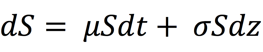
In this article, Jayati WALIA (ESSEC Business School, Grande Ecole Program – Master in Management, 2019-2022) explains how implied volatility is computed from option market prices and a option pricing model.

Introduction

Volatility is a measure of fluctuations observed in an asset’s returns over a period of time. The standard deviation of historical asset returns is one of the measures of volatility. In option pricing models like the Black-Scholes-Merton model, volatility corresponds to the volatility of the underlying asset’s return. It is a key component of the model because it is not directly observed in the market and cannot be directly computed. Moreover, volatility has a strong impact on the option value.

Mathematically, in a reverse way, implied volatility is the volatility of the underlying asset which gives the theoretical value of an option (as computed by Black-Scholes-Merton model) equal to the market price of that option.

Implied volatility is a forward-looking measure because it is a representation of expected price movements in an underlying asset in the future.

Computation methods for implied volatility

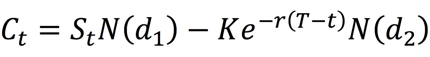
The Black-Scholes-Merton (BSM) model provides an analytical formula for the price of both a call option and a put option.

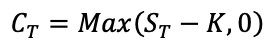
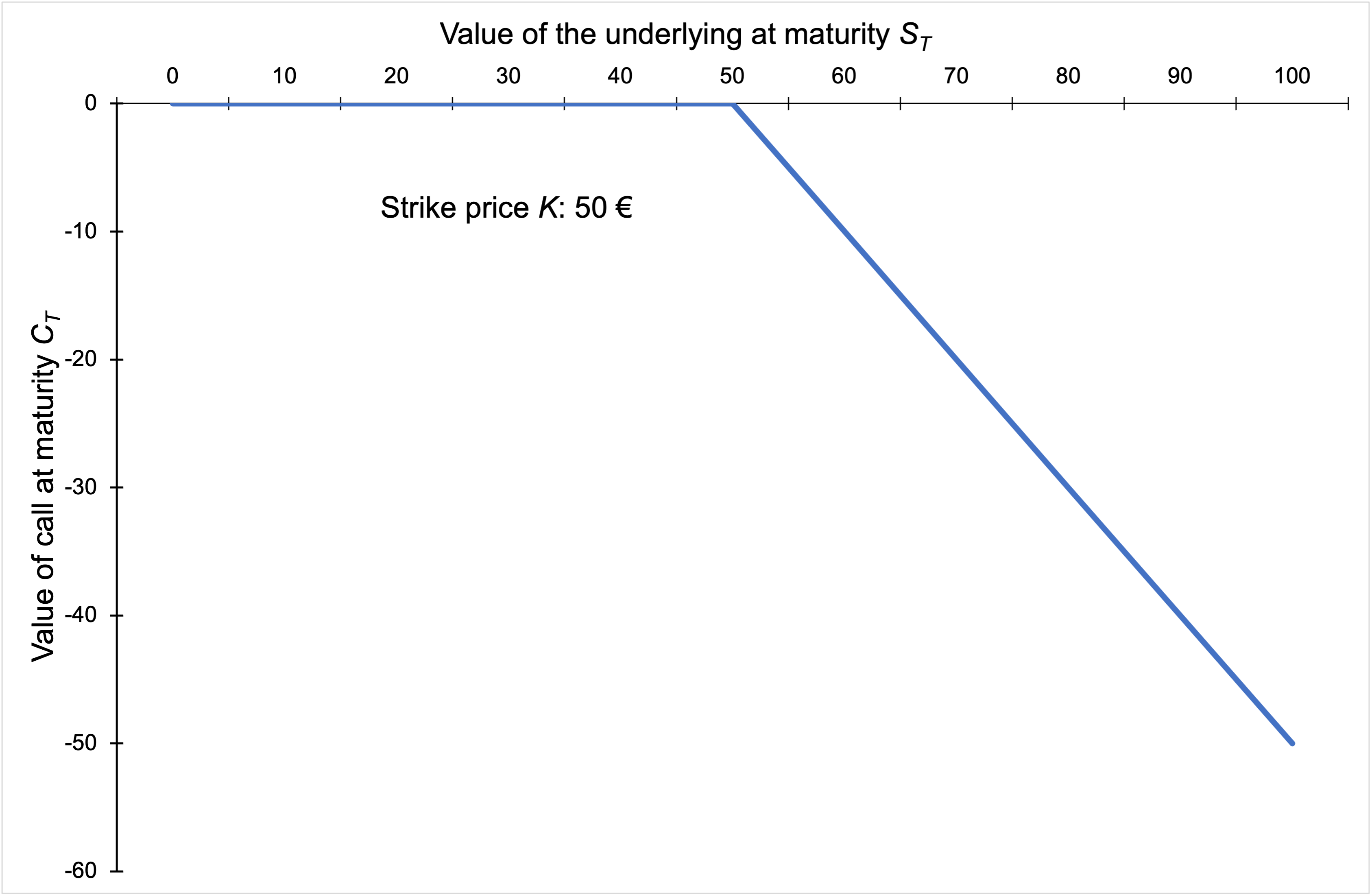
The value for a call option at time t is given by:

Call option value

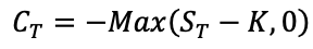
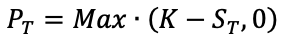
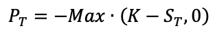
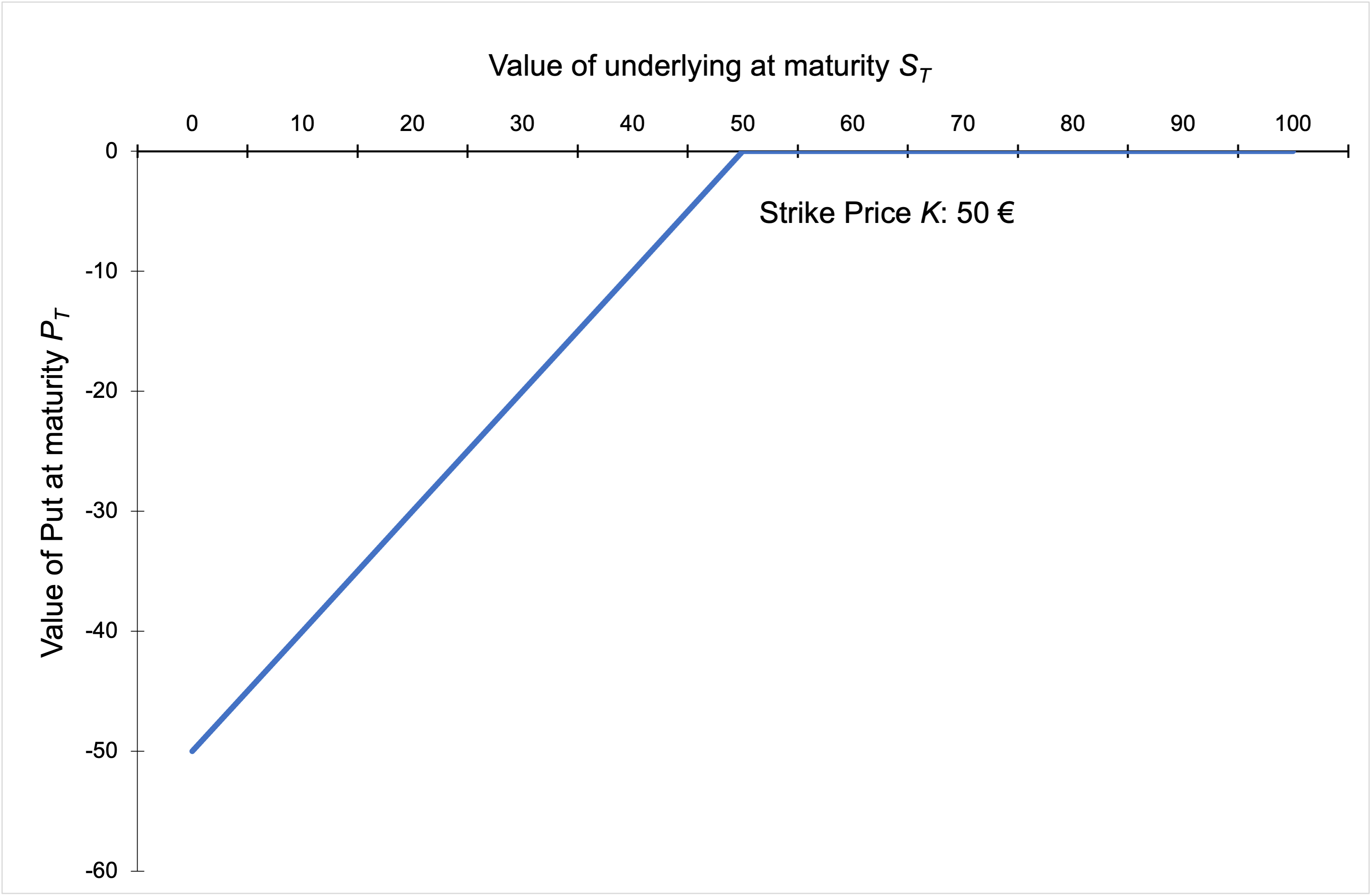
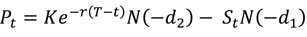
The value for a put option at time t is given by:

Put option value

where the parameters d₁ and d₂ are given by:,

call option d1 d2

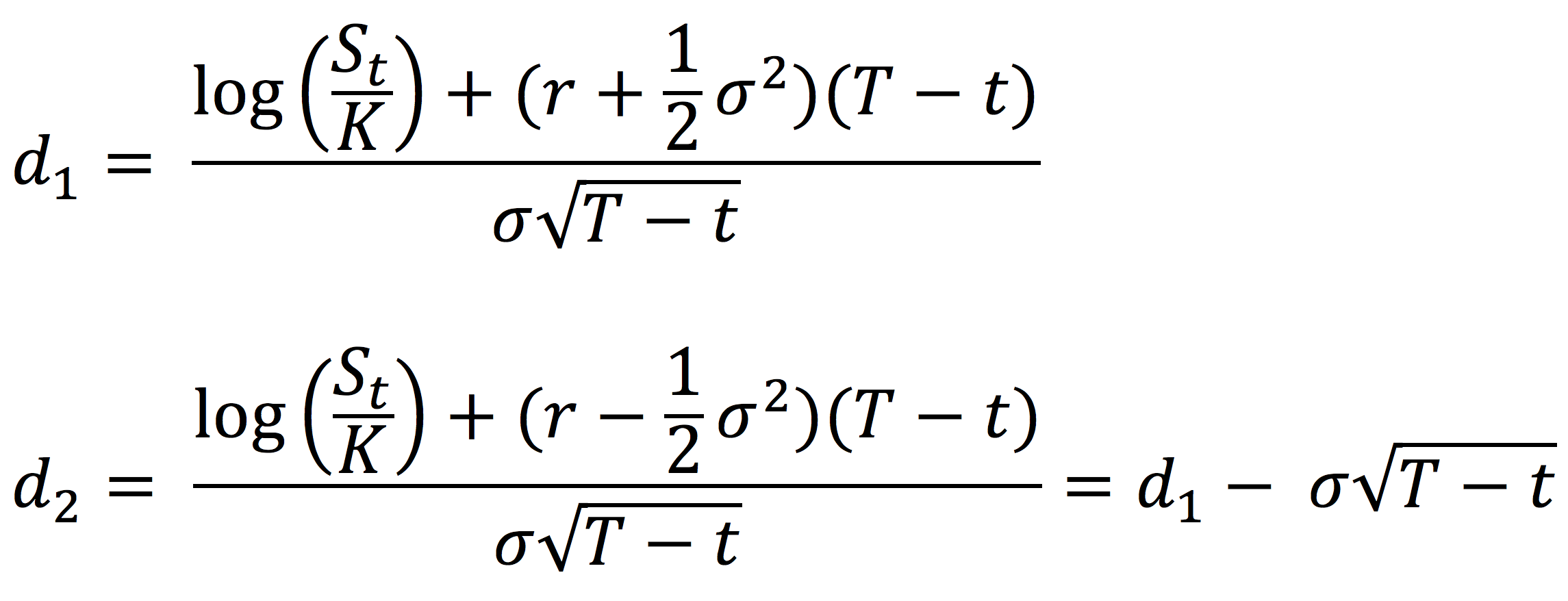
with the following notations:

S_t : Price of the underlying asset at time t
t: Current date
T: Expiry date of the option
K: Strike price of the option
r: Risk-free interest rate
σ: Volatility of the underlying asset
N(.): Cumulative distribution function for a normal (Gaussian) distribution. It is the probability that a random variable is less or equal to its input (i.e. d₁ and d₂) for a normal distribution. Thus, 0 ≤ N(.) ≤ 1

From the BSM model, both for a call option and a put option, the option price is an increasing function of the volatility of the underlying asset: an increase in volatility will cause an increase in the option price.

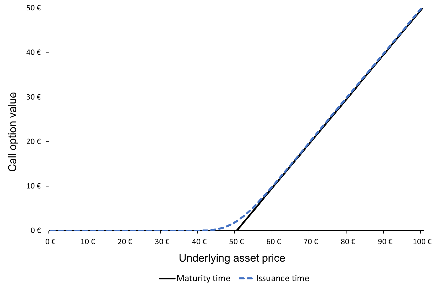
Figures 1 and 2 below illustrate the relationship between the value of a call option and a put option and the level of volatility of the underlying asset according to the BSM model.

Figure 1. Call option value as a function of volatility.

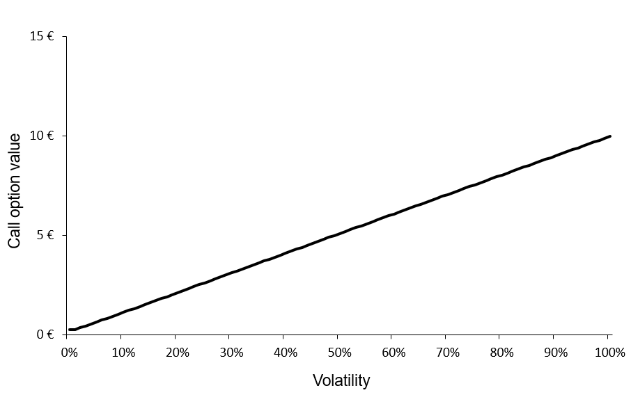
Source: computation by the author (BSM model)

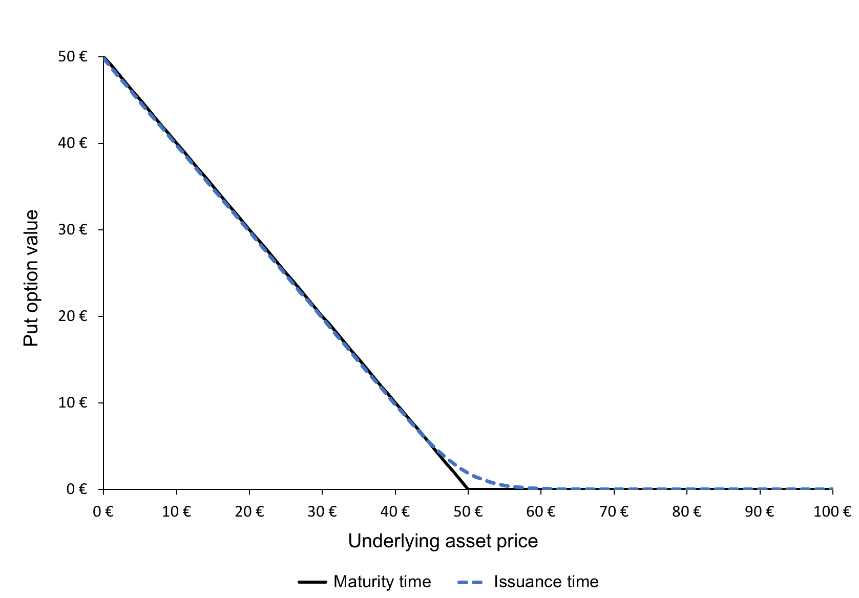
Figure 2. Put option value as a function of volatility.

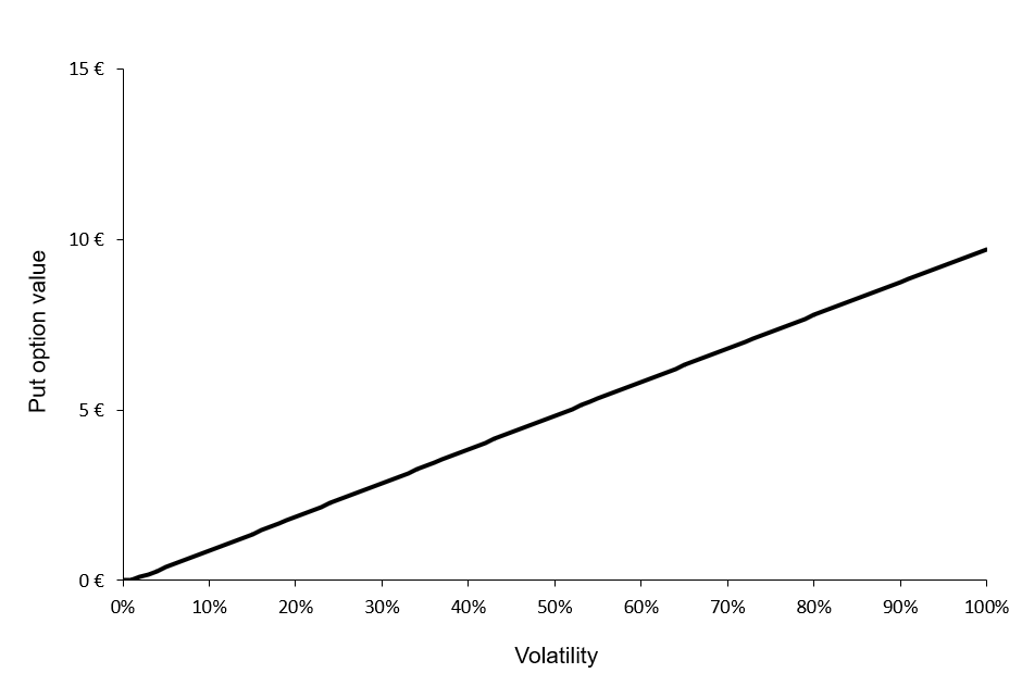
Source: computation by the author (BSM model)

You can download below the Excel file for the computation of the value of a call option and a put option for different levels of volatility of the underlying asset according to the BSM model.

We can observe that the call and put option values are a monotonically increasing function of the volatility of the underlying asset. Then, for a given level of volatility, there is a unique value for the call option and a unique value for the put option. This implies that this function can be reversed; for a given value for the call option, there is a unique level of volatility, and similarly, for a given value for the put option, there is a unique level of volatility.

The BSM formula can be reverse-engineered to compute the implied volatility i.e., if we have the market price of the option, the market price of the underlying asset, the market risk-free rate, and the characteristics of the option (the expiration date and strike price), we can obtain the implied volatility of the underlying asset by inverting the BSM formula.

Example

Consider a call option with a strike price of 50 € and a time to maturity of 0.25 years. The market risk-free interest rate is 2% and the current price of the underlying asset is 50 €. Thus, the call option is ‘at-the-money’. If the market price of the call option is equal to 2 €, then the associated level of volatility (implied volatility) is equal to 18.83%.

You can download below the Excel file below to compute the implied volatility given the market price of a call option. The computation uses the Excel solver.

Volatility smile

Volatility smile is the name given to the plot of implied volatility against different strikes for options with the same time to maturity. According to the BSM model, it is a horizontal straight line as the model assumes that the volatility is constant (it does not depend on the option strike). However, in practice, we do not observe a horizontal straight line. The curve may be in the shape of the alphabet ‘U’ or a ‘smile’ which is the usual term used to refer to the observed function of implied volatility.

Figure 3 below depicts the volatility smile for call options on the Apple stock on May 13, 2022.

Figure 3. Volatility smile for call options on Apple stock.
Apple volatility smile
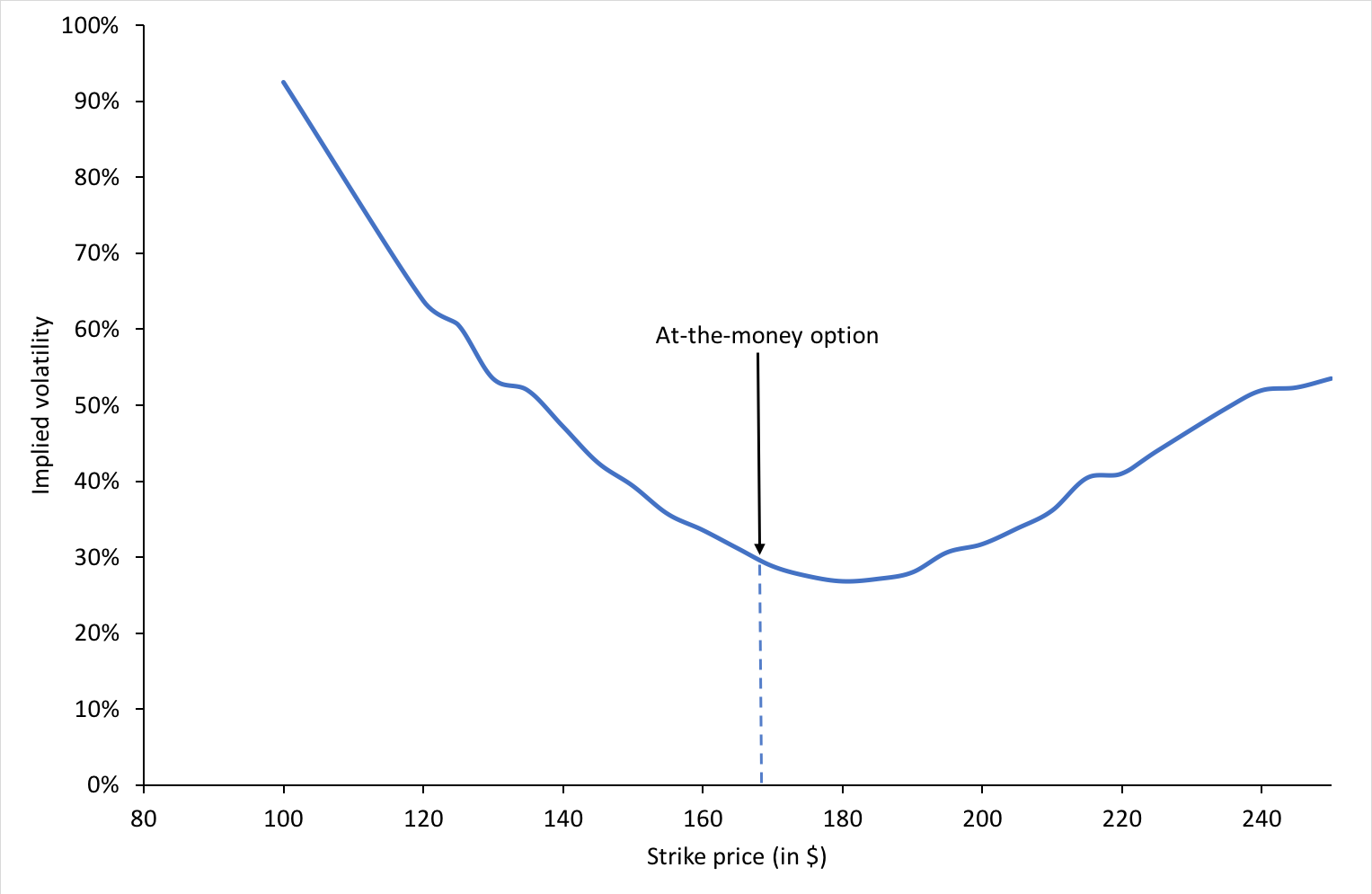
Source: Computation by author.

We can also observe that the for a specific time to maturity, the implied volatility is minimum when the option is at-the-money.

Volatility surface

An essential assumption of the BSM model is that the returns of the underlying asset follow geometric Brownian motion (corresponding to log-normal distribution for the price at a given point in time) and the volatility of the underlying asset price remains constant over time until the expiration date. Thus theoretically, for a constant time to maturity, the plot of implied volatility and strike price would be a horizontal straight line corresponding to a constant value for volatility.

Volatility surface is obtained when values for implied volatilities are calculated for options with different strike prices and times to maturity.

CBOE Volatility Index

The Chicago Board Options Exchange publishes the renowned Volatility Index (also known as VIX) which is an index based on the implied volatility of 30-day option contracts on the S&P 500 index. It is also called the ‘fear gauge’ and it is a representation of the market outlook for volatility for the next 30 days.

Useful resources

Academic articles

Black F. and M. Scholes (1973) “The Pricing of Options and Corporate Liabilities” The Journal of Political Economy, 81, 637-654.

Dupire B. (1994). “Pricing with a Smile” Risk Magazine 7, 18-20.

Merton R.C. (1973) “Theory of Rational Option Pricing” Bell Journal of Economics, 4, 141–183.

Business

CBOE Volatility Index (VIX)

CBOE VIX tradable products

About the author

The article was written in May 2022 by Jayati WALIA (ESSEC Business School, Grande Ecole Program – Master in Management, 2019-2022).

Black-Scholes-Merton option pricing model

February 4, 2024March 3, 2022 by Jayati WALIA

In this article, Jayati WALIA (ESSEC Business School, Grande Ecole Program – Master in Management, 2019-2022) explains the Black-Scholes-Merton model to price options.

The Black-Scholes-Merton model (or the BSM model) is the world’s most popular option pricing model. Developed in the beginning of the 1970s, this model introduced to the world, a mathematical way of pricing options. Its success was essentially a starting point for new forms of financial derivatives in the knowledge that they could be priced accurately using the ideas and analyses pioneered by Black, Scholes and Merton and it set the foundation for the flourishing of modern quantitative finance. Myron Scholes and Robert Merton were awarded the Nobel Prize for their work on option pricing in 1997. Unfortunately, Fischer Black had died several years earlier but would certainly have been included in the prize had he been alive, and he was also listed as a contributor by Scholes and Merton.

Today, the Black-Scholes-Merton formula is widely used by traders in investment banks to price and hedge option contracts. Options are used by investors to hedge their portfolios to manage their risks.

Assumptions of the BSM Model

As any model, the BSM model relies on a set of assumptions:

The model considers European options, which we can only be exercised at their expiration date.
The price of the underlying asset follows a geometric Brownian motion (corresponding to log-normal distribution for the price at a given point in time).
The risk-free rate remains constant over time until the expiration date.
The volatility of the underlying asset price remains constant over time until the expiration date.
There are no dividend payments on the underlying asset.
There are no transaction costs on the underlying asset.
There are no arbitrage opportunities.

The BSM equation

The value of an option is a function of the price of the underlying stock and its statistical behavior over the life of the option.

A commonly used model is Geometric Brownian Motion (GBM). GBM assumes that future asset price differences are uncorrelated over time and the probability distribution function of the future prices is a log-normal distribution (or equivalently the probability distribution function of the future returns is a normal distribution). The price movements in a GBM process can be expressed as:

GBM equation

with dS being the change in the underlying asset price in continuous time dt and dX the random variable from the normal distribution (N(0, 1) or Wiener process). σ is the volatility of the underlying asset price (it is assumed to be constant). μdt represents the deterministic return within the time interval with μ representing the growth rate of asset price or the ‘drift’.

Therefore, option price is determined by these parameters that describe the process followed by the asset price over a period of time. The Black-Scholes-Merton equation governs the price evolution of European stock options in financial markets. It is a linear parabolic partial differential equation (PDE) and is expressed as:

BSM model equation

Where V is the value of the option (as a function of two variables: the price of the underlying asset S and time t), r is the risk-free interest rate (think of it as the interest rate which you would receive from a government debt or similar debt securities) and σ is the volatility of the log returns of the underlying security (say stocks).

The key idea behind the equation is to hedge the option and limit exposure to market risk posed by the asset. This is achieved by a strategy known as ‘delta hedging’ and it involves replicating the option through an equivalent portfolio with positions in the underlying asset and a risk-free asset in the right way so as to eliminate risk.

Thus, from the BSM equation we can derive the BSM formulae that describe the price of call and put options over their life time.

The BSM formulae

Note that the type of option we are valuing (call or put), the strike price and the maturity date do not appear in the above BSM equation. These elements only appear in the ‘final condition’ i.e., the option value at maturity, called the payoff function.

For a call option, the payoff C is given by:

C_T = max⁡(S_T – K; 0)

For a put option, the payoff is given by:

P_T = max⁡(K – S_T; 0)

The BSM formula is a solution to the BSM equation, given the boundary conditions (given by the payoff equations above). It calculates the price at time t for both a call and a put option.

The value for a call option at time t is given by:

Call option value equation

The value for a put option at time t is given by:

Put option value equation

where

With the notations:
S_t: Price of the underlying asset at time t
t: Current date
T: Expiry date of the option
K: Strike price of the option
r: Risk-free interest rate
σ: Volatility (the standard deviation of the return on the underlying asset)
N(.): Cumulative distribution function for a normal (Gaussian) distribution. It is the probability that a random variable is less or equal to its input (i.e. d₁ and d₂) for a normal distribution. Thus, 0 ≤ N(.) ≤ 1

Figure 1 gives the graphical representation of the value of a call option at time t as a function of the price of the underlying asset at time t as given by the BSM formula. The strike price for the call option is 50€ with a maturity of 0.25 years and volatility of 50% in the underlying.

Figure 1. Call option value

Source: computation by author.

Figure 2 gives the graphical representation of the value of a put option at time t as a function of the price of the underlying asset at time t as given by the BSM formula. The strike price for the put option is 50€ with a maturity of 0.25 years and volatility of 50% in the underlying.

Figure 2. Put option value
Source: computation by author.

You can download below the Excel file for option pricing with the BSM Model.

Some Criticisms and Limitations

American options

The Black-Scholes-Merton model was initially developed for European options. This is a limitation of the equation for American options which can be exercised at any time before the expiry date. The BSM model would then not accurately determine the option value (an important case when the underlying asset pays a discrete dividend).

Stocks paying dividends

Also, in reality, most stocks pay dividends, and no dividends was an assumption in the initial BSM model, which analysts now eliminated by accommodating the dividend yield in the formula if required.

Constant volatility

Another limitation is the use of constant volatility. Volatility is the measure of risk based on the standard deviation of the return on the underlying asset. In reality the value of an asset will change randomly, not with a specific constant pattern regarding the way it can change.

Finally, the assumption of no transaction cost neglects the liquidity risk in the market since transaction costs are clearly incurred in the real world and there exists a bid-offer spread on most underlying assets. For the most heavily traded stocks, this cost may be low but for others it may lead to an inaccuracy.

Useful resources

Black F. and M. Scholes (1973) The Pricing of Options and Corporate Liabilities The Journal of Political Economy 81, 637-654.

Merton R.C. (1973) Theory of Rational Option Pricing Bell Journal of Economics 4, 141–183.

About the author

The article was written in March 2022 by Jayati WALIA (ESSEC Business School, Grande Ecole Program – Master in Management, 2019-2022).

Protective Put

January 12, 2022 by Akshit GUPTA

Protective Put

This article written by Akshit GUPTA (ESSEC Business School, Grande Ecole Program – Master in Management, 2019-2022) presents the concept of protective put using option contracts.

Introduction

Hedging is a strategy implemented by investors to reduce the risk in an existing investment. In financial markets, hedging is an effective tool used by investors to minimize the risk exposure and change the risk profile for any investment in securities. While hedging does not necessarily eliminate the entire risk for any investment, it does limit the potential losses that the investor can incur.

Option contracts are commonly used by market participants (traders, investors, asset managers, etc.) as hedging mechanisms due to their great flexibility (in terms of expiration date, moneyness, liquidity, etc.) and availability. Positions in options are used to offset the risk exposure in the underlying security, another option contract or in any other derivative contract. There are various popular strategies that can be implemented through option contracts to minimize risk and maximize returns, one of which is a protective put.

Buying a protective put

A put option gives the buyer of the option, the right but not the obligation, to sell a security at a predefined date and price.

A protective put also called as a synthetic long option, is a hedging strategy that limits the downside of an investment. In a protective put, the investor buys a put option on the stock he/she holds in its portfolio. The protective put option acts as a price floor since the investor can sell the security at the strike price of the put option if the price of the underlying asset moves below the strike price. Thus, the investor caps its losses in case the underlying asset price moves downwards. The investor has to pay an option premium to buy the put option.

The maximum payoff potential from using this strategy is unlimited and the potential downside/losses is limited to the strike price of the put option.

Market scenario

A put option is generally bought to safeguard the investment when the investor is bullish about the market in the long run but fears a temporary fall in the prices of the asset in the short term.

For example, an investor owns the shares of Apple and is bullish about the stock in the long run. However, the earnings report for Apple is due to be released by the end of the month. The earnings report can have a positive or a negative impact on the prices of the Apple stock. In this situation, the protective put saves the investor from a steep decline in the prices of the Apple stock if the report is unfavorable.

Let us consider a protective position with buying at-the money puts. One of following three scenarios may happen:

Scenario 1: the stock price does not change, and the puts expire at the money.

In this scenario, the market viewpoint of the investor does not hold correct and the loss from the strategy is the premium paid on buying the put options. In this case, the option holder does not exercise its put options, and the investor gets to keep the underlying stocks.

Scenario 2: the stock price rises, and the puts expire in the money.

In this scenario, since the price of the stock was locked in through the put option, the investor enjoys a short-term unrealized profit on the underlying position. However, the put option will not be exercised by the investor and it will expire worthless. The investor will lose the premium paid on buying the puts.

Scenario 3: the stock price falls, and the puts expire out of the money.

In this scenario, since the price of the stock was locked in through the put option, the investor will execute the option and sell the stocks at the strike price. There is protection from the losses since the investor holds the put option.

Risk profile

In a protective put, the total cost of the investment is equal to the price of the underlying asset plus the put price. However, the profit potential for the investment is unlimited and the maximum losses are capped to the put option price. The risk profile of the position is represented in Figure 1.

Figure 1. Profit or Loss (P&L) function of the underlying position and protective put position.

Protective put

Source: computation by the author.

You can download below the Excel file for the computation of the Profit or Loss (P&L) function of the underlying position and protective put position.

The delta of the position is equal to the sum of the delta of the long position in the underlying asset (+1) and the long position in the put option (Δ). The delta of a long put option is negative which implies that a fall in the asset price will result in an increase in the put price and vice versa. However, the delta of a protective put strategy is positive. This implies that in a protective put strategy, the value of the position tends to rise when the underlying asset price increases and falls when the underlying asset prices decreases.

Figure 2 represents the delta of the protective put position as a function of the price of the underlying asset. The delta of the put option is computed with the Black-Scholes-Merton model (BSM model).

Figure 2. Delta of a protective put position.
Delta Protective put
Source: computation by the author (based on the BSM model).

You can download below the Excel file for the computation of the delta of a protective put position.

Example

An investor holds 100 shares of Apple bought at the current price of $144 each. The total initial investment is equal to $14,400. He is skeptical about the effect of the upcoming earnings report of Apple by the end of the current month. In order to avoid losses from a possible downside in the price of the Apple stock, he decides to purchase at-the-money put options on the Apple stock (lot size is 100) with a maturity of one month, using the protective put strategy.

We use the following market data: the current price of Appel stock is $144, the implied volatility of Apple stock is 22.79% and the risk-free interest rate is equal to 1.59%.

Based on the Black-Scholes-Merton model, the price of the put option $3.68.

Let us consider three scenarios at the time of maturity of the put option:

Scenario 1: stability of the price of the underlying asset at $144

The market value of the investment $14,400. The total cost of the initial investment is the cost of acquiring the Apple stocks ($14,400) plus the cost of buying the put options ($368 = $3.68*100), which is equal to $14,768, (i.e. ($14,400 + $368)).

As the stock price is stable at $144, the investor will not execute the put option and the option will expire worthless.

By not executing the put option, the investor incurs a loss which is equal to the price of the put option which is $368.

Scenario 2: an increase in the price of the underlying asset to $155

The market value of the investment $15,500. The total cost of the initial investment is the cost of acquiring the Apple stocks ($14,400) plus the cost of buying the put options ($368 = $3.68*100), which is equal to $14,768, (i.e. ($14,400 + $368)).

As the stock price is at $155, the investor will not execute the put option and hold on the underlying stock.

By not executing the put option, the investor incurs a loss which is equal to the price of the put option which is $368.

Scenario 3: a decrease in the price of the underlying asset to $140

The market value of the investment $14,000. The total cost of the initial investment is the cost of acquiring the Apple stocks ($14,400) plus the cost of buying the put options ($368 = $3.68*100), which is equal to $14,768, (i.e. ($14,400 + $368)).

As the stock price has decreased to $140, the investor will execute the put option and sell the Apple stocks at $144. By executing the put option, the investor will protect himself from incurring a loss of $400 (i.e.($144-$140)*100) due to a decrease in the Apple stock prices.

▶ All posts about Options

▶ Akshit GUPTA Options

▶ Akshit GUPTA The Black-Scholes-Merton model

▶ Akshit GUPTA Option Greeks – Delta

▶ Akshit GUPTA Covered call

▶ Akshit GUPTA Option Trader – Job description

Useful Resources

Black F. and M. Scholes (1973) “The Pricing of Options and Corporate Liabilities” The Journal of Political Economy, 81, 637-654.

Hull J.C. (2015) Options, Futures, and Other Derivatives, Ninth Edition, Chapter 10 – Trading strategies involving Options, 276-295.

Merton R.C. (1973) “Theory of Rational Option Pricing” Bell Journal of Economics, 4(1): 141–183.

Wilmott P. (2007) Paul Wilmott Introduces Quantitative Finance, Second Edition, Chapter 8 – The Black Scholes Formula and The Greeks, 182-184.

About the author

Article written in January 2022 by Akshit GUPTA (ESSEC Business School, Grande Ecole Program -Master in Management, 2019-2022).

Understanding Options and Options Trading Strategies

December 13, 2021 by Luis RAMIREZ

Understanding Options and Options Trading Strategies

In this article, Luis RAMIREZ (ESSEC Business School, Global BBA, 2019-2023) discusses the fundamentals behind options trading.

Financial derivatives

In order to understand and grasp the concept of options, knowledge of what is a derivative should be established. A financial instrument derivative is ultimately an instrument whose value derives from the value of an underlying asset (or multiple underlying assets). These underlying assets can of course be bonds, stocks, commodities, currencies, etc. Derivatives are widely common and used around the world; investment banks, commercial banks, and corporations (mainly multinational corporations) are all consistent users of derivatives. The purpose, or goal, behind derivatives is to manage risk, whether that be alleviating risk by hedging investments, or by taking on risk through speculative investments. To carry out this process, the investor must undertake one of the four types of derivatives. The four types are the following: options, forwards, futures, and swaps. In this article the focus will be solely placed on options.

What are options?

An option contract provides an investor the chance to either buy (for a call option) or sell (for a put option) the underlying asset, depending on what type of option they possess. Every option contract has an expiry date in which the investor can effectively exercise the option. A very important thing about options is that they provide investors the right, but not the obligation, to either buy or sell an asset (i.e., stock shares) at a price and at a date that have been agreed at the issuing of the cotnract.

Put options vs call options

Firstly, the main two different options are call and put options. Call options give investors (that bought the call option) the right to buy a stock at a certain price and at a certain date, and put options give investors (that bought the put option) the right to sell a stock at a certain price and at a certain date. The first step into acquiring options, either type, is paying a premium. This premium which is spent at the beginning of the process is the only loss that investors will face if the options are not exercised. However, the other side of the coin, options writers (sellers) are more exposed to risk as they are exposed to lose more than only the premium.

Sell-side vs buy-side

In an option contract, the price at which the asset is sold or bought is known as the strike price, or exercise price. When a call option has been bought, and the price of the share has
had a bullish trend and rises above the strike price, the investor can simply exercise his right to buy the share at the strike price, and then immediately sell it at the spot price, resulting in immediate profit. However, if the price of the share had a bearish trend and dropped below the strike price, the investor can decide not to exercise his right and will only lose the amount of premium paid in this case.

Figure 1. Profit and loss (P&L) of a long position in a call option
as a function of the price of the underlying asset at maturity
Profit and loss (P&L) as a function of the price of the underlying asset at maturity

Profit and loss (P&L) as a function of the price of the underlying asset at maturity

Source: production by the author.

On the other hand, selling options differs. Selling options is commonly known as writing options. The way this works is that a writer receives the premium from a buyer, this is the maximum profit a writer can receive by selling call options. Normally, a call option writer is bearish, therefore he believes that the price of the stack will fall below that of the strike price. If indeed the share price falls below the strike price, the writer would profit the premium paid by the buyer, since the buyer would not exercise the option. However, if the share price surpassed the strike price, the writer would have to sell shares at the low strike price. The writer would then experience a loss, the size of the loss depends on how many shares and price the writer would have to use to cover the entire option contract. Clearly, the risk for call writers is much higher than the risk exposure call buyers when acquiring an option. To summarize, the call buyer can only lose the premium paid, and the call writer can face infinite risk because the price of a share can keep increasing.

Figure 2. Profit and loss (P&L) of a short position in a call option
as a function of the price of the underlying asset at maturity
Profit and loss (P&L) as a function of the price of the underlying asset at maturity

Source: production by the author.

As for put options, put buyers usually believe the share price will decrease under the strike price. If this does eventually happen, the investor can simply exercise the put and sell at strike price, instead of a lower spot price. If the investor wants to go long, he can substitute the shares used in the option contract and buy them for a cheaper spot price after the put has been exercised. However, if the spot price is above the strike price, and the investor choses to not exercise the put, the loss will once again only be the cost of the premium.

Figure 3. Profit and loss (P&L) of a long position in a put option
as a function of the price of the underlying asset at maturity
Profit and loss (P&L) as a function of the price of the underlying asset at maturity

Source: production by the author.

On the other hand, put writers think the share price will have a bullish trend throughout the duration of the option lifecycle. If the share price rises above strike price, the contract will expire, and the seller’s profit is the premium he received. If the share price decreases, and falls under the strike price, then the writer is obliged to buy shares at a strike price which higher than the spot price. This is when the risk is at the highest for a put writer, if the share price falls. Just like call writing, the loss can be hefty. Only that in the case of put writing, it happens if the share price tumbles down.

Figure 4. Profit and loss (P&L) of a short position in a put option
as a function of the price of the underlying asset at maturity
Profit and loss (P&L) as a function of the price of the underlying asset at maturity

Source: production by the author.

This can be shrunk down to knowing that call buyers can benefit from buying securities or assets at a lower price if the share price rises during the length of the option contract. Put buyers can benefit from selling assets at a higher strike price if the share price falls during the length of the option contract. As per writers, they receive a premium fee when writing options. However, it is not all positive points, option buyers need to pay the premium fee and discount this from their potential profit, and writers face an indefinite risk subject to the share price and quantity.

Figure 5. Market scenarios for buying and selling call and put options

Source: production by the author.

Option Trading Strategies

Four trading strategies have already been mentioned, selling or buying either puts or calls. However, there are several different option trading strategies and new ones are being produced frequently, anyhow the article will focus on five trading strategies that most, if not all, investors are familiar with.

Covered Call

This trading strategy consists in the writer selling call options against the stock that he already owns. It is ‘covered’ because it covers the writer when the buyer of the option exercises his right to buy the shares, due to the writer already owning them, meaning that the writer can deliver the shares. This strategy is often used as an income stream from premiums. This is an employable strategy for those who believe that the asset they own will only experience a small change in price. The covered call is considered a low-risk strategy, and if used appropriately with a reliable stock, it can be a source of income.

Figure 6. Profit and loss (P&L) of a covered call
as a function of the price of the underlying asset at maturity

Source: production by the author.

Married put

Like a covered call, in a married put the investor buys an asset and then buys a put option with the strike price being equal to the spot price. This is done to be protected against a decrease in the asset price. Of course, when buying an option, a premium must be paid, which is a downside for a married put strategy. However, the married put limits the loss an investor could incur in case of a price decrease. On the other hand, if the price increases, profit is unlimited. This strategy is often used for volatile stocks.

Figure 7. Profit and loss (P&L) of a married put
as a function of the price of the underlying asset at maturity

Source: production by the author.

Protective Collar

This strategy is done when an investor buys a put option where the strike price is lower than the spot price, as well as instantly writing a call option where the strike price is higher than the spot price, this must be done by the investor owning said asset. This strategy protects the investor from a decrease in price. If the share price increases, large profits will be capped, however large losses will be also capped. When performing a protective collar, the best possibility for an investor is that the share price rises to the call strike price.

Figure 8. Profit and loss (P&L) of a protective collar
as a function of the price of the underlying asset at maturity

Source: production by the author.

Bull Call Spread

In order to execute this strategy, an investor buys calls at the same time that he sells the equivalent order of calls, which have a higher strike price. Of course, both calls must be tied to the same asset. As seen on the name of this strategy, it is a strategy that an investor employs when he predicts a bullish trend. Just like the protective collar, it limits both, gains and losses.

Figure 9. Profit and loss (P&L) of a bull call spread
as a function of the price of the underlying asset at maturity

Source: production by the author.

Bear Put Spread

This strategy is like the Bull Call Spread, only that it is in terms of a put option. The investor buys put options while he sells put options at a lower strike price. This can be done when the investor foresees a bearish trend, just like its call counterpart, the Bear Put Spread limits losses and gains.

Figure 10. Profit and loss (P&L) of a bear put spread
as a function of the price of the underlying asset at maturity

Source: production by the author.

Importance of options on financial markets

As seen on the variety of option trading strategies, and the different factors that play into each strategy mentioned, and dozens of other out there to explore, this instrument is a very utilized tool for investors, and financial institutions. The ‘options within options’ are of a huge variety and so much could be done. Many people have strong feelings towards this derivative, whether it is a negative, or positive stance, it all depends on the profits it brings. There is a lot of work behind options, and just like any other investment, due diligence is a key aspect of the procedure.

Useful Resources

Hull J.C. (2015) Options, Futures, and Other Derivatives, Ninth Edition.

Prof. Longin’s website Pricer d’options standards sur actions – Calls et puts (in French)

About the author

Article written in December 2021 by Luis RAMIREZ (ESSEC Business School, Global BBA, 2019-2023).

Hedging strategies – Equities

September 19, 2021 by Akshit GUPTA

Hedging Strategies – Equities

This article written by Akshit GUPTA (ESSEC Business School, Master in Management, 2019-2022) presents the different hedging strategies based on option contracts.

Introduction

Hedging is a risk mitigation strategy used by investors reduce the risk in an existing investment. In financial markets, hedging is used as an effective tool by investors to minimize the risk exposure and maximize the returns for any investment in securities. Equity options are commonly used by investors / traders as hedging mechanisms due to their great flexibility (in terms of expiration date, moneyness, liquidity, etc.) and availability. Hedging does not eliminate the entire risk for any investment but often limits the potential losses that the investor can incur. Positions in equity options are used to offset the risk exposure in the underlying equity, another option contract or in any other derivative contract.

Different strategies used in hedging

There are many ways to hedge the exposure in any given security. Some of the most used hedging strategies for an exposure in equity includes the following:

Writing a covered call

A call option gives the buyer of the option, the right but not the obligation, to buy a security at a fixed date and price defined in the contract. In a covered call, the investor writes (sells) a call option on the stock he holds in his portfolio. He earns the premium by writing the call option. Investors execute this strategy when they are bullish about the stock. The maximum payoff potential from this strategy is limited but the potential downside/losses is can be quite high (although limited).

Covered call

Buying a protective put

A put option gives the buyer of the option, the right but not the obligation, to sell a security at a fixed date and price defined in the contract. In a protective put, the investor buys a put option on the stock she holds in her portfolio. She pays the premium by buying the put option. Investors execute this strategy when they are bearish about the stock. The maximum payoff potential from this strategy is unlimited but the potential downside/losses is limited.

Protective Put

Spreads

Spreads are option hedging strategies where the investor/trader will take positions in multiple options of the same type (either call options or put options on the same underlying). The different types of spreads are mentioned below:

Strangle and Straddle

In a strangle, the investor buys a European call and a European put option, both at the same expiration date but different strike prices. To benefit from this strategy, the price of the underlying asset must move further away from the central value in either direction i.e., increase or decrease. If the stock prices stay at a level closer to the central value, the investor will incur losses. This strategy is suitable for investors who expect a huge price movement but are unsure of the direction of the movement.

Strangle

In a straddle, the investor buys a European call and a European put option, both at the same expiration date and at the same strike price. This strategy works in a similar manner like a strangle. However, the potential losses are a bit higher than incurred in a strangle if the stock price remains near the central value at expiration date.

Straddle

Bull and Bear spreads

In a bull spread, the investor buys a European call option on a stock with strike price K1 and sells a call option on the same stock at strike price K2 (which is higher than K1) at the same expiration date. The investor forecasts the prices to go up and is bullish about the stock. The spread limits the potential downside risk on buying the call option, but also limits the potential profit by capping the upside. It Is used as an effective hedge to limit the losses.

Bull spread

In a bear spread, the investor expects the prices of the stock to decline. In order to hedge against the downside, the investor buys a put option at strike price K2 and sells a put option at strike price K1, where K1 < K2. Initially, this strategy leads to a cash outflow since the put option is sold at a lower strike price, which results in lower premium.

Bear spread

Useful Resources

Hull J.C. (2015) Options, Futures, and Other Derivatives, Ninth Edition, Chapter 10 – Trading strategies involving Options, 276-295.

Investopedia Using Options as a Hedging Strategy

▶ Gupta A. Option Greeks – Delta

▶ Gupta A. History of Options markets

▶ Gupta A. Option Trader – Job description

▶ Gupta A. Options

About the author

Article written in September 2021 by Akshit GUPTA (ESSEC Business School, Master in Management, 2019-2022).

Types of exercise for option contracts

February 5, 2024September 19, 2021 by Akshit GUPTA

Types of exercise for option contracts

This article written by Akshit GUPTA (ESSEC Business School, Grande Ecole Program – Master in Management, 2019-2022) presents the different types of exercise for option contracts.

Introduction

Exercising a call option contract means the purchase of the underlying asset by the call buyer at the price set in the option contract (strike price). Similarly, exercising a put option contract means the sale of the underlying asset by the put buyer at the price set in the option contract.

The different option contracts can be settled in cash or with a physical delivery of the underlying asset. Normally, the equity, fixed interest security and commodity option contracts are settled using physical delivery and index options are settled in cash.

Majority of options are not exercised before the maturity date because it is not optimal for the option holder to do so. Note that for options with physical delivery, it may be better to close the position before the expiration date). If an option expires unexercised, the option holder loses any of the rights granted in the contract (indeed, in-the-money options are automatically exercised at maturity). Exercising options is a sophisticated and at times a complicated process and option holder need to take several factors into consideration while making the decision about exercise such as opinion about future market behavior of underlying asset in option, tax implications of exercise, net profit that will be acquired after deducting exercise commissions, option type, vested shares, etc.

Different types of exercise for option contracts

The option style does not deal with the geographical location of where they are traded! The contracts differ in terms of their expiration time when they can be exercised. The option contracts can be categorized as per different styles they come in. Some of the most common styles of option contracts are:

American options

American-style options give the option buyer the right to exercise his/her option anytime prior or up to the expiration date of the contract. These options provide greater flexibility to the option buyer but also come at a higher price as compared to the European-style options.

European options

European-style options can only be exercised on the expiration or maturity date of the contract. Thus, they offer less flexibility to the option buyer. However, the European options are cheaper as compared to the American options.

Bermuda options

Bermuda options are a mix of both American and European style options. These options can only be exercised on specific predetermined dates or periods up to the expiration date. They are considered to be exotic option contracts and provide limited flexibility to the option buyer.

Early Exercise

Early exercise is a strategy of exercising options before the expiration date and is possible with American options only. The question is: when the holder of an American option should exercise his/her option? Before the expiration date or at the expiration date? Quantitative models say that it could be optimal to exercise American options before the date of a dividend payout (options are not protected against the payement of dividends by firms) and sometimes for deep in-the-money put options.

There are many strategies that investors follow while exercising option contracts in order to maximize their gains and hedge risks. A few of them are discussed below:

Exercise-and-Hold

Investors can purchase their option shares with cash and hold onto them. This allows them to benefit from ownership in company stock, providing potential gains from any increase in stock value and dividend payments if any. Investors are also liable to pay brokerage commissions fees and taxes.

Exercise-and-Sell

This is a cashless strategy wherein investors purchase the option shares and then immediately sell them. Brokerages generally allow this kind of transaction without use of cash, with the money from the stock sale covering the purchase price, as well as the commissions and taxes associated with the transaction. This choice provides investors with available cash in pocket to invest elsewhere too.

Exercise-and-Sell-to-Cover

In this strategy too, investors exercise the option and then immediately sell enough shares to cover the purchase price, commissions fees and taxes. The remaining shares remain with the investor.

Useful Resources

Academic research

Hull J.C. (2015) Options, Futures, and Other Derivatives, Ninth Edition, Chapter 10 – Mechanics of options markets, 235-240.

Business analysis

Fidelity Exercising Stock Options

About the author

Article written in August 2021 by Akshit GUPTA (ESSEC Business School, Grande Ecole Program – Master in Management, 2019-2022).

Options

February 4, 2024June 20, 2021 by Akshit GUPTA

Options

This article written by Akshit GUPTA (ESSEC Business School, Grande Ecole Program – Master in Management, 2019-2022) presents an introduction to Options.

Introduction

Options is a type of derivative which gives the buyer of the option contract the right, but not the obligation, to buy (for a call option) or sell (for a put option) an underlying asset at a price which is pre-determined, and a date set in the future.

Option contracts can be traded between two or more counterparties either over the counter or on an exchange, where the contracts are listed. Exchange based trading of option contracts was introduced to the larger public in April 1973, when Chicago Board Options Exchange (CBOE)) was introduced in the US. The options market has grown ever since with over 50 exchanges that trade option contracts worldwide.

Terminology used for an option contract

The different terms that are used in an option contract are:

Option Spot price

The option spot price is the price at which the option contract is trading at the time of entering the contract.

Underlying spot price

The underlying spot price is the price at which the underlying asset is trading at the time of entering the option contract.

Strike price

Strike price is essentially the price at which the option buyer can exercise his/her right to buy or sell the option contract at or before the expiration date. The strike price is pre-determined at the time of entering the contract.

Expiration date

The expiration date is the date at which the option contracts ends or after which it becomes void. The expiration date of an option contract can be set to be after weeks, months or year.

Lot size

A lot size is the quantity of the underlying asset contained in an option contract. The size is decided and amended by the exchanges from time to time. For example, an Option contract on an APPLE stock trading on an exchange in USA consists of 100 underlying APPLE stocks.

Option class

Option class is the type of option contracts that the trader is trading on. It can be a Call or a Put option.

Position

The position a trader can hold in an option contract can either be Long or Short depending on the strategy. A Long position essentially means Buying the option and a short position means Selling or writing the option contract.

Option Premium

Option premium is the price at which the option contracts trade in the market.

Benefits of using an option contract

Trading in option contracts gives the traders certain benefits which can be categorised as:

Hedging Benefits

Hedging is an essential benefit of the option contract. For an investor or a trader holding an underlying stock, an option contract provides them with the opportunity to offset their risk exposure by buying or selling an option contract as per their market outlook. If an trader holding stocks of APPLE is bearish about the market and expects the market to fall, he/she can buy a PUT option which essentially gives him/her the right to sell the security at a pre-determined price and date. Such a contract protects the trader from significant losses which he/she might incur if the stock price for APPLE goes down significantly.

Cost Benefits

While buying an option contract, the traders benefits from the leverage effect which exchanges across the world provides. Leverage helps the traders to multiply the size of their holdings with lesser capital investment. This also helps them to earn higher profits by taking limited risks.

Choice Benefits

In traditional trading, traders have a limited degree of flexibility as they can only buy or sell assets based on their outlook. Whereas, Option contracts provides a great choice to the traders as they can take different positions in call and put options (Long and short positions) and for different strikes and maturities.
They can also use different strategies and spreads to execute and manage their positions to earn profits.

Types of option contracts

The option contracts can be broadly classified into two categories: call options and put options.

Call options

A call option is a derivative contract which gives the holder of the option the right, but not an obligation, to buy an underlying asset at a pre-determined price on a certain date. An investor buys a call option when he believes that the price of the underlying asset will increase in value in the future. The price at which the options trade in an exchange is called an option premium and the date on which an option contract expires is called the expiration date or the maturity date.

For example, an investor buys a call option on Apple shares which expires in 1 month and the strike price is $90. The current apple share price is $100. If after 1 month,
The share price of Apple is $110, the investor exercises his rights and buys the Apple shares from the call option seller at $90.

But, if the share prices for Apple falls to $80, the investor doesn’t exercise his right and the option expires because the investor can buy the Apple shares from the open market at $80.

Put options

A put option is a derivative contract which gives the holder of the option the right, but not an obligation, to sell an underlying asset at a pre-determined price on a certain date. An investor buys a put option when he believes that the price of the underlying asset will decrease in value in the future.

For example, an investor buys a put option on Apple shares which expires in 1 month and the strike price is $110. The current apple share price is $100. If after 1 month,
The share price of Apple is $90, the investor exercises his rights and sell the Apple shares to the put option seller at $110.
But, if the share prices for Apple rises to $120, the investor doesn’t exercise his right and the option expires because the investor can sell the Apple shares in the open market at $120.

Different styles of option exercise

The option style doesn’t deal with the geographical location of where they are traded. However, the contracts differ in terms of their expiration time when they can be exercised. The option contracts can be categorized as per different styles they come in. Some of the most common styles of option contracts are:

American options

American style options give the option buyer the right to exercise his option any time prior or up to the expiration date of the contract. These options provide greater flexibility to the option buyer but also comes at a high price as compared to the European style options.

European options

European style options can only be exercised on the expiration or maturity date of the contract. Thus, they offer less flexibility to the option buyer in terms of his rights. However, the European options are cheaper as compared to the American options.

Bermuda options

Bermuda options are a mix of both American and European style options. These options can only be exercised on a specific pre-determined dates up to the expiration date. They are considered to be exotic option contracts and provide limited flexibility to the option buyer to exercise his claim.

Different underlying assets for an option contract

The different underlying assets for an option contract can be:

Individual assets: stocks, bonds

Option traders trading in individual assets can take positions in call or put options for equities and bonds based on the reports provided by the research teams. They can take long or short positions in the option contract. The positions depend on the market trends and individual asset analysis. The option contracts on individual assets are traded in different lot sizes.

Indexes: stock indexes, bond indexes

Options traders can also trade on contracts based on different indexes. These contracts can be traded over the counter or on an exchange. These traders generally follow the macroeconomic trends of different geographies and trade in the indices based on specific markets or sectors. For example, some of the most known exchange traded index options are options written on the CAC 40 index in France, the S&P 500 index and the Dow Jones Industrial Average Index in the US, etc.

Foreign currency options

Different banks and investment firms deal in currency hedges to mitigate the risk associated with cross border transactions. Options traders at these firms trade in foreign currency option contracts, which can be over the counter or exchange traded.

Option Positions

Option traders can take different positions depending on the type of option contract they trade. The positions can include:

Long Call

When a trader has a long position in a call option it essentially means that he has bought the call option which gives the trader the right to buy the underlying asset at a pre-determined price and date. The buyer of the call option pays a price to the option seller to buy the right and the price is called the Option Premium. The maximum loss to a call option buyer is restricted to the amount of the option premium he/she pays.

Long Call

With the following notations:
   C_T = Call option value at maturity T
   S_T = Price of the underlying at maturity T
   K = Strike price of the call option

The graph of the payoff of a long call is depicted below. It gives the value of the long position in a call option at maturity T as a function of the price of the underlying asset at time T.

Payoff of a long position in a call option
Long call

Short Call

When a trader has a short position in a call option it essentially means that he has sold the call option which gives the buyer of the option the right to buy the underlying asset from the seller at a pre-determined price and date. The seller of the call option is also called the option writer and he/she receive a price from the option buyer called the Option Premium. The maximum gain to a call option seller is restricted to the amount of the option premium he/she receives.

Short call

With the following notations:
   C_T = Call option value at maturity T
   S_T = Price of the underlying at maturity T
   K = Strike price of the call option

The graph of the payoff of a short call is depicted below. It gives the value of the short position in a call option at maturity T as a function of the price of the underlying asset at time T.

Payoff of a short position in a call option
Short call

Long Put

When a trader has a long position in a put option it essentially means that he/she has bought the put option which gives the trader the right to sell the underlying asset at a pre-determined price and date. The buyer of the put option pays a price to the option seller to buy the right and the price is called the Option Premium. The maximum loss to a put option buyer is restricted to the amount of the option premium he/she pays.

Long Put

With the following notations:
   P_T = Put option value at maturity T
   S_T = Price of the underlying at maturity T
   K = Strike price of the put option

The graph of the payoff of a long put is depicted below. It gives the value of the long position in a put option at maturity T as a function of the price of the underlying asset at time T.

Payoff of a long position in a put option
Long put

Short Put

When a trader has a short position in a put option it essentially means that he has sold the call option which gives the buyer of the option the right to sell the underlying asset from the seller at a pre-determined price and date. The seller of the put option is also called the option writer and he/she receive a price from the option buyer called the Option Premium. The maximum gain to a put option seller is restricted to the amount of the option premium he/she receives.

Short Put

With the following notations:
   P_T = Put option value at maturity T
   S_T = Price of the underlying at maturity T
   K = Strike price of the put option

The graph of the payoff of a short put is depicted below. It gives the value of the short position in a put option at maturity T as a function of the price of the underlying asset at time T.

Payoff of a short position in a put option
Short put

Useful Resources

Academic research

Hull J.C. (2015) Options, Futures, and Other Derivatives, Ninth Edition, Chapter 10 – Mechanics of options markets, 235-240.

Business analysis

CNBC Live option trading for APPLE stocks

About the author

Article written in June 2021 by Akshit GUPTA (ESSEC Business School, Grande Ecole Program – Master in Management, 2019-2022).

History of Options Markets

February 4, 2024June 20, 2021 by Akshit GUPTA

History of the options markets

This article written by Akshit GUPTA (ESSEC Business School, Grande Ecole Program – Master in Management, 2019-2022) presents an introduction to the History of the Options markets.

Introduction

Options are a type of derivative contracts which give the buyer the right, but not the obligation, to buy or sell an underlying security at a pre-determined price and date. These contracts can either be traded over-the-counter (OTC) through dealer or broker network or can be traded over an exchange in a standardized form.

A brief history

The history of the use of options can be dated back to ancient times. In early 4th century BC, a philosopher, and an astronomer, named Thales of Miletus calculated a surplus olive harvest in his region during the period. He predicted an increase in demand for the olive presses due to an increase in the harvest. To benefit from his prediction, he bought the rights to use the olive presses in his region by paying a certain sum. The olive harvest saw a significant surplus that year and the demand for olive presses rose, as predicted by him. He then exercised his option and sold the rights to use the olive presses at a much higher prices than what he actually paid, making a good profit. This is the first documented account of the use of option contracts dating back to 4th century BC.

The use of option contracts was also seen during the Tulip mania of 1636. The tulip producers used to sell call options to the investors when the tulip bulbs were planted. The investors had the right to buy the tulips, when they were ready for harvest, at a price pre-determined while buying the call option. However, since the markets were highly unstandardized, the producers could default on their obligations.
But the event laid a strong foundation for the use of option contracts in the future.

Until 1970s, option contracts were traded over-the-counter (OTC) between investors. However, these contracts were highly unstandardized leading to investor distrust and illiquidity in the market.

In 1973, the Chicago Board Options Exchange (CBOE)) was formed in USA, laying the first standardized foundation in options trading. In 1975, the Options clearing corporation (OCC) was formed to act as a central clearing house for all the option contracts that were traded on the exchange. With the introduction of these 2 important bodies, the option trading became highly standardized and general public gained access to it. However, the Put options were introduced only in 1977 by CBOE. Prior to that, only Call options were traded on the exchange.

With the advent of time, options market grew significantly with more exchanges opening up across the world. The option pricing models, and risk management strategies also became more sophisticated and complex.

Market participants

The participants in the options markets can be broadly classified into following groups:

Market makers: A market maker is a market participant in the financial markets that simultaneously buys and sells quantities of any option contract by posting limit orders. The market maker posts limit orders in the market and profits from the bid-ask spread, which is the difference by which the ask price exceeds the bid price. They play a significant role in the market by providing liquidity.
Margin traders: Margin traders are market participants who make use of the leverage factor to invest in the options markets and increase their position size to earn significant profits. But this trading style is highly speculative and can also lead to high losses due to the leverage effect.
Hedgers: Investors who try to reduce their exposure in the financial markets by using hedging strategies are called hedgers. Hedgers often trades in derivative products to offset their risk exposure in the underlying assets. For example, a hedger who is bearish about the market and has shares of Apple, will buy a Put option on the shares of Apple. Thus, he has the right to sell the shares at a high price if the market price for apple shares goes down.
Speculators: Speculative investors are involved in option trading to take advantage of market movements. They usually speculative on the price of an underlying asset and account for a significant share in option trading.

Types of option contracts

The option contracts can be broadly classified into two main categories, namely:

Call options

But, if the share prices for Apple falls to $80, the investor doesn’t exercise his right and the option expires because the investor can buy the Apple shares from the open market at $80.

Put options

For example, an investor buys a put option on Apple shares which expires in 1 month and the strike price is $110. The current apple share price is $100. If after 1 month,

The share price of Apple is $90, the investor exercises his rights and sell the Apple shares to the put option seller at $110.

But, if the share prices for Apple rises to $120, the investor doesn’t exercise his right and the option expires because the investor can sell the Apple shares in the open market at $120.

Different style of options

American options

European options

Bermuda options

Useful Resources

Chapter 10 – Mechanics of options markets, pg. 235-240, Options, Futures, and Other Derivatives by John C. Hull, Ninth Edition

Wikipedia Options (Finance)

The Street A Brief History of Stock Options

About the author

Article written in June 2021 by Akshit GUPTA (ESSEC Business School, Grande Ecole Program – Master in Management, 2019-2022).

Introduction

Computation methods for implied volatility

Example

Volatility smile

Volatility surface

CBOE Volatility Index

Related posts on the SimTrade blog

Useful resources

Academic articles

Business

About the author

Assumptions of the BSM Model

The BSM equation

The BSM formulae

Some Criticisms and Limitations

American options

Stocks paying dividends

Constant volatility

Related posts on the SimTrade blog

Useful resources

About the author

Protective Put

Introduction

Buying a protective put

Market scenario

Scenario 1: the stock price does not change, and the puts expire at the money.

Scenario 2: the stock price rises, and the puts expire in the money.

Scenario 3: the stock price falls, and the puts expire out of the money.

Risk profile

Example

Scenario 1: stability of the price of the underlying asset at $144

Scenario 2: an increase in the price of the underlying asset to $155

Scenario 3: a decrease in the price of the underlying asset to $140

Related Posts

Useful Resources

About the author

Understanding Options and Options Trading Strategies

Financial derivatives

What are options?

Put options vs call options

Sell-side vs buy-side

Option Trading Strategies

Covered Call

Married put

Protective Collar

Bull Call Spread

Bear Put Spread

Importance of options on financial markets

Related posts on the SimTrade blog

Useful Resources

About the author

Hedging Strategies – Equities

Introduction

Different strategies used in hedging

Writing a covered call

Buying a protective put

Spreads

Strangle and Straddle

Bull and Bear spreads

Useful Resources

Related Posts

About the author

Types of exercise for option contracts

Introduction

Different types of exercise for option contracts

American options

European options

Bermuda options

Early Exercise

Exercise-and-Hold

Exercise-and-Sell

Exercise-and-Sell-to-Cover

Related posts on the SimTrade blog

Useful Resources

Academic research

Business analysis

About the author

Options

Introduction

Terminology used for an option contract