In this article, Saral BINDAL (Indian Institute of Technology Kharagpur, Metallurgical and Materials Engineering, 2024-2028 & Research assistant at ESSEC Business School) presents two statistical models used in finance to describe the time behavior of asset prices: the arithmetic Brownian motion (ABM) and the geometric Brownian motion (GBM).
Introduction
In financial markets, performance over time is governed by three fundamental variables: the drift (μ), volatility (σ), and maybe most importantly time (T). The drift represents the expected growth rate of the price and corresponds to the expected return of assets or portfolios. Volatility measures the uncertainty or risk associated with price fluctuations around this expected growth and corresponds to the standard deviation of returns. The relationship between these variables reflects the trade-off between risk and return. Time, which is related to the investment horizon set by the investor, determines how both performance and risk accumulate. Together, these variables form the foundation of asset pricing to model the behavior of market price over time, and in fine the performance of the investor at their investment horizon.
Modeling asset prices
Asset price modeling is used to understand the expected return and risk in asset management, risk management, and the pricing of complex financial products such as options and structured products. Although asset prices are influenced by countless unpredictable risk factors, quants in finance always try to find a parsimonious way to model asset prices (using a few parameters only).
The first study of asset price modelling dates from Louis Bachelier in 1900, in his doctoral thesis Théorie de la Spéculation (The Theory of Speculation), where he modelled stock prices as a random walk and applied this framework to option valuation. Later, in 1923, the mathematician Norbert Wiener formalized these ideas as the Wiener process, providing the rigorous stochastic foundation that underpins modern finance.
In the 1960s, Paul Samuelson refined Bachelier’s model by introducing the geometric Brownian motion, which ensures positive stock prices following a lognormal statistical distribution. His 1965 paper “Rational Theory of Warrant Pricing” laid the groundwork for modern asset price modelling, showing that discounted stock prices follow a martingale.
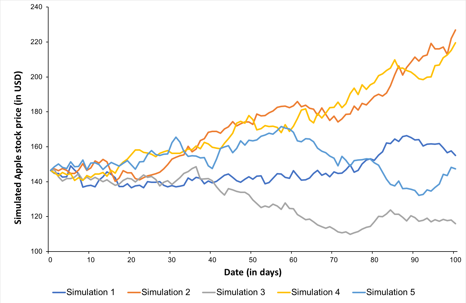
We detail below the two models usually used in finance to model the evolution of asset prices over time: the arithmetic Brownian motion (ABM) and the geometric Brownian motion (GBM). We will then use these models to simulate the evolution of asset prices over time with the Monte Carlo simulation method.
Arithmetic Brownian motion (ABM)
Theory
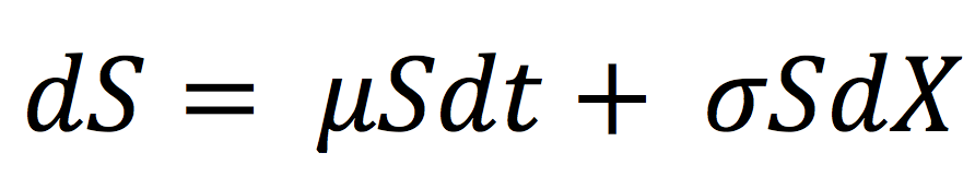
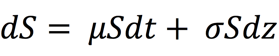
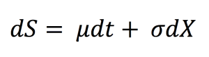
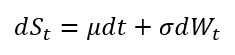
One of the most widely used stochastic processes in financial modeling is the arithmetic Brownian motion, also known as the Wiener process. It is a continuous stochastic process with normally distributed increments. Using the Wiener process notation, an asset price model in continuous time based on an ABM can be expressed as the following stochastic differential equation (SDE):
where:
- dSt = infinitesimal change in asset price at time t t
- μ = drift (growth rate of the asset price)
- σ = volatility (standard deviation)
- dWt = infinitesimal increment of wiener process (N(0,dt))
Note that the standard Brownian motion is a special case of the arithmetic Brownian motion with a mean equal to zero and a variance equal to one.
In this model, both μ and σ are assumed to be constant over time. It can be shown that the probability distribution function of the future price is a normal distribution implying a strictly positive (although negligible in most cases) probability for the price to be negative.
Integrating the SDE for dSt over a finite interval (from time 0 to time t), we get:
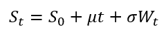
Here, Wt is defined as Wt = √t · Zt, where Zt is a normal random variable drawn from the standard distribution N(0, 1) with mean equal to 0 and variance equal to 1.
At any date t, we can also compute the expected value and a confidence interval such that the asset price St lies between the lower and upper bound of the interval with probability equal to 1-α.
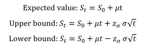
Where S0 is the initial asset price and zα.
The z-score for a confidence level of (1 – α) can be calculated as:
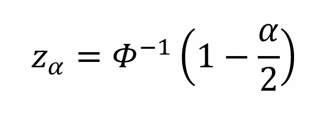
where Φ-1 denotes the inverse cumulative distribution function (CDF) of the standard normal distribution.
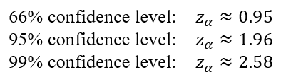
For example the statistical z-score (zα) values for 66%, 95%, and 99% confidence intervals are as the following:
Monte Carlo simulations with ABM
Since Monte Carlo simulations are performed in discrete time, the underlying continuous-time asset price process (ABM) is approximated using the Euler–Maruyama discretization of SDEs (see Maruyama, 1955), as shown below.
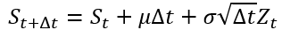
where Δt denotes the time step, expressed in the same time units as the drift parameter μ and the volatility parameter σ (usually the annual unit). For example, Δt may be equal to one day (=1/252) or one month (=1/12).
Figure 1 below illustrates a single simulated asset price path under an arithmetic Brownian motion (ABM), sampled at monthly intervals (Δt = 1/12) over a 10-year horizon (T = 10). Alongside the simulated path, the figure shows the expected (mean) price trajectory and the corresponding upper and lower bounds of a 66% confidence interval. In this example, the model assumes an annual drift (μ) of $8, representing the expected growth rate, and an annual volatility (σ) of $15, capturing random price fluctuations. The initial asset price (S0) is equal to $100.
Figure 1. Single Monte Carlo–simulated asset price path under an Arithmetic Brownian Motion model.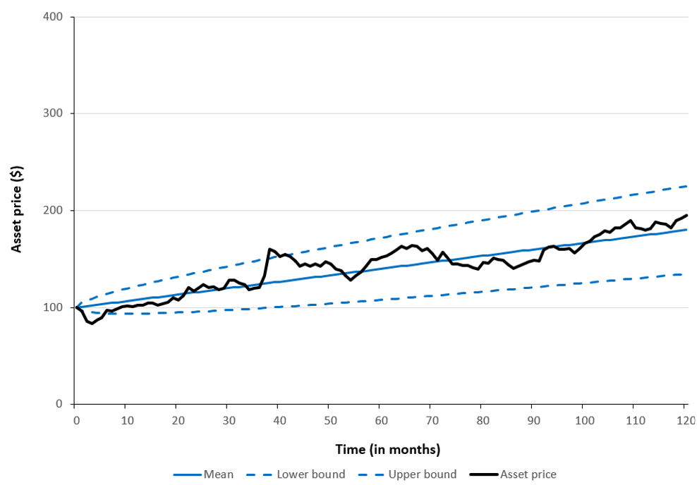
Source: computation by the author (with Excel).
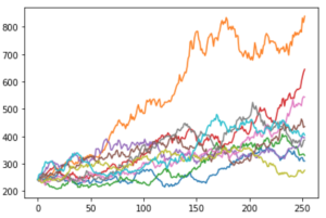
Figure 2 below illustrates 1,000 simulated asset price paths generated under an arithmetic Brownian motion (ABM). In addition to the simulated paths, the figure displays the expected (mean) price trajectory along with the corresponding upper and lower bounds of a 66% confidence interval, using the same parameter settings as in Figure 1.
Figure 2. Monte Carlo–simulated asset price paths under an Arithmetic Brownian Motion model.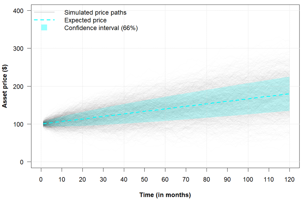
Source: computation by the author (with R).
Geometric Brownian motion (GBM)
Theory
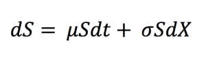
Since an arithmetic Brownian motion (ABM) can take negative values, it is unsuitable for directly modeling stock prices if we assume limited liability for investors. Under limited liability, an investor’s maximum possible loss is indeed confined to their initial investment, implying that asset prices cannot fall below zero. To address this limitation, financial models instead use geometric Brownian motion (GBM), a non-negative stochastic process that is widely employed to describe the evolution of asset prices. Using the Wiener process notation, an asset price model in continuous time based on a GBM can be expressed as the following stochastic differential equation (SDE):
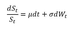
where:
- St = asset price at time t t
- μ = drift (growth rate of the asset price)
- σ = volatility (standard deviation)
- dWt = infinitesimal increment of wiener process (N(0,dt))
Integrating the SDE for dSt/St over a finite interval, we get:
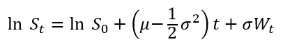
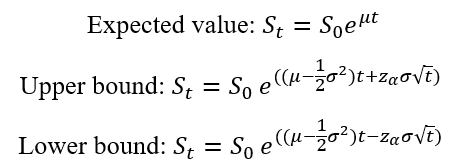
The theoretical expected value and confidence intervals are given analytically by the following expressions:
Monte Carlo simulations with GBM
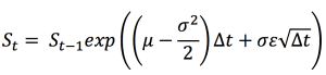
To implement Monte Carlo simulations, we approximate the underlying continuous-time process in discrete time, yielding:
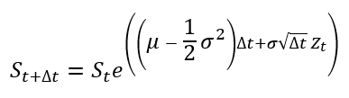
where Zt is a standard normal random variable drawn from the distribution N(0, 1) and Δt denotes the time step, chosen so that it is expressed in the same time units as the drift parameter μ and the volatility parameter σ.
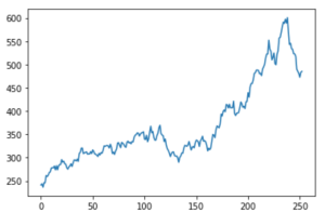
Figure 3 below illustrates a single simulated asset price path under a geometric Brownian motion (GBM), sampled at monthly intervals (Δt = 1/12) over a 10-year horizon (T = 10). Alongside the simulated path, the figure shows the expected (mean) price trajectory and the corresponding upper and lower bounds of a 66% confidence interval. In this example, the model assumes an annual drift (μ) of 8%, representing the expected growth rate, and an annual volatility (σ) of 15%, capturing random price fluctuations. The initial asset price is S0 €100.
Figure 3. Monte Carlo–simulated asset price path under a Geometric Brownian Motion model.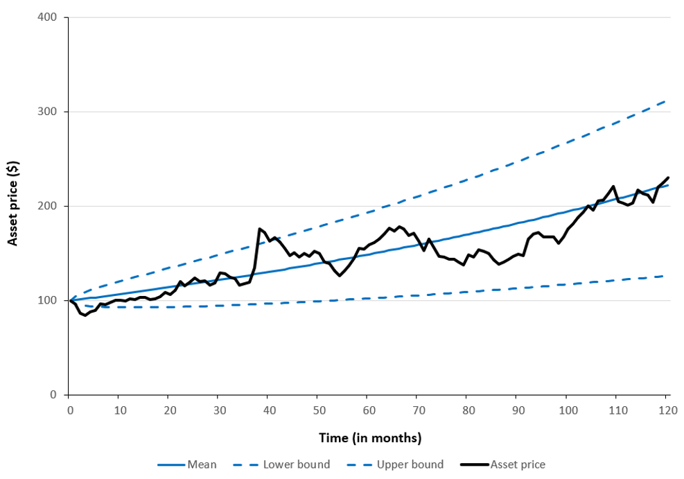
Source: computation by the author (with Excel).
Figure 4 below illustrates 1,000 simulated asset price paths generated under a geometric Brownian motion (GBM). In addition to the simulated paths, the figure displays the expected (mean) price trajectory along with the corresponding upper and lower bounds of a 66% confidence interval, using the same parameter settings as in Figure 3.
Figure 4. Monte Carlo–simulated asset price paths under a Standard Brownian Motion model.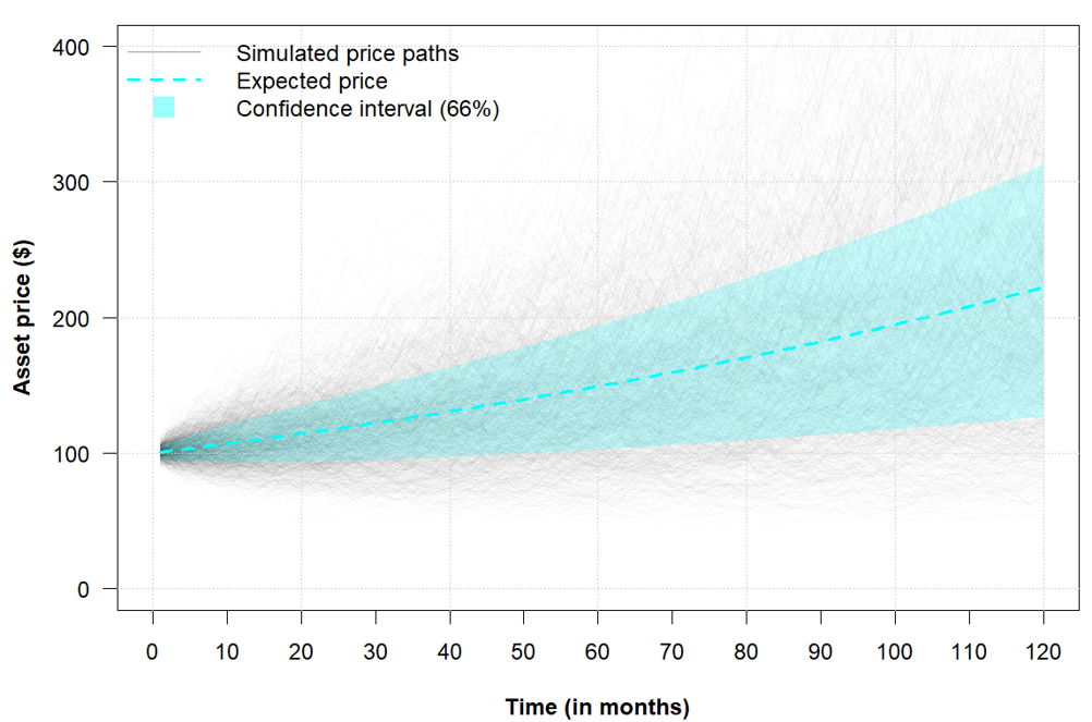
Source: computation by the author (with R).
Discussion
The drift μ represents the expected rate of growth of asset prices, so its cumulative contribution increases linearly with time as μT. In contrast, volatility σ captures investment risk, and its cumulative impact scales with the square root of time as σ√T. As a result, over short horizons stochastic shocks tend to dominate the deterministic drift, whereas over longer horizons the expected growth component becomes increasingly prominent.
When many paths for the asset price are simulated and plotted over time, the resulting trajectories form a cone-shaped region, commonly referred to as a fan chart. The center of this fan traces the smooth expected path governed by the drift μ, while the widening envelope reflects the growing dispersion of outcomes induced by volatility σ.
This representation underscores a key implication for long-term investing and risk management: uncertainty expands with the investment horizon even when model parameters remain constant. While the expected value evolves predictably and linearly through time, the range of plausible outcomes broadens at a slower, square-root rate, shaping the risk–return trade-off across different time scales.
You can download the Excel file provided below for generating Monte Carlo Simulations for asset prices modeled on arithmetic and geometric Brownian motion.

You can download the Python code provided below, for generating Monte Carlo Simulations for asset prices modeled on arithmetic and geometric Brownian motion.

Alternatively, you can download the R code below with the same functionality as in the Python file.

Link between the ABM and the GBM
The ABM and GBM models are fundamentally different: the drift for the ABM is additive while the drift for the GBM is multiplicative. Moreover, the statistical distribution for the price for the ABM is a normal distribution while the statistical distribution for the GBM is a log-normal distribution. However, we can study the relationship between the two models as they are both used to model the same phenomenon, the evolution of asset prices over time in our case.
We can especially study the relationship between the two parameters of the two models, μ and σ. In the presentation above, we used the same notations for μ and σ for the two models, but the values of these parameters for the two models will be different when we apply these models to the same phenomenon. There is no mapping of the ABM and GBM in the price space such that we get the same results as the two models are fundamentally different.
Let us rewrite the two models (in terms of SDE) by differentiating the parameters for each model:
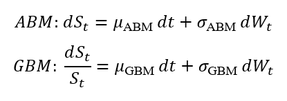
To model the same phenomenon, we can use the following relationship between the parameters of the ABM and GBM models:
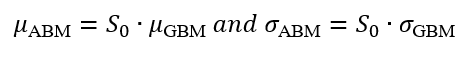
To make the two models comparable in terms of price behavior, an ABM can locally approximate GBM by matching instantaneous drift and volatility such that:
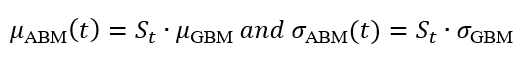
This local correspondence is state-dependent and time-varying, and therefore not a true parameter equivalence.
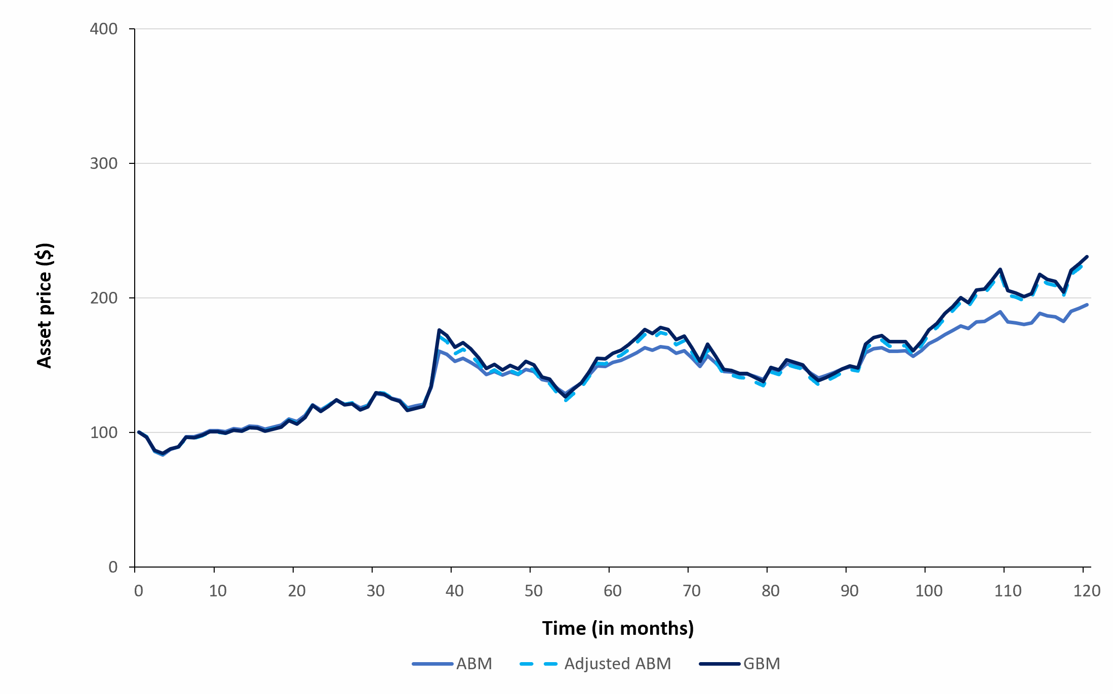
Figure 5 below compares the asset price path for an ABM, monthly adjusted ABM and a GBM.
Why should I be interested in this post?
Understanding how asset prices are modeled, and in particular the difference between additive and multiplicative price dynamics, is essential for building strong intuition about how prices evolve over time under uncertainty. This understanding forms the foundation of modern risk management, as it directly informs concepts such as capital protection, downside risk, and the long-term behavior of investment portfolios.
Related posts on the SimTrade blog
▶ Saral BINDAL Historical Volatility
▶ Saral BINDAL Implied Volatility and Option Prices
▶ Jayati WALIA Brownian Motion in Finance
▶ Jayati WALIA Monte Carlo simulation method
Useful resources
Academic research
Bachelier L. (1900) Théorie de la spéculation. Annales scientifiques de l’École Normale Supérieure, 3e série, 17, 21–86.
Kataoka S. (1963) A stochastic programming model. Econometrica, 31, 181–196.
Lawler G.F. (2006) Introduction to Stochastic Processes, 2nd Edition, Chapman & Hall/CRC, Chapter “Brownian Motion”, 201–224.
Maruyama G. (1955) Continuous Markov processes and stochastic equations. Rendiconti del Circolo Matematico di Palermo, 4, 48–90.
Samuelson P.A. (1965) Rational theory of warrant pricing. Industrial Management Review, 6(2), 13–39.
Telser L. G. (1955) Safety-first and hedging. Review of Economic Studies, 23, 1–16.
Wiener N. (1923) Differential-space. Journal of Mathematics and Physics, 2, 131–174.
Other
H. Hamedani, Brownian Motion as the Limit of a Symmetric Random Walk, ProbabilityCourse.com Online chapter section.
About the author
The article was written in January 2026 by Saral BINDAL (Indian Institute of Technology Kharagpur, Metallurgical and Materials Engineering, 2024-2028 & Research assistant at ESSEC Business School).
▶ Discover all articles written by Saral BINDAL