Saral BINDAL, Author at SimTrade blog

Measures and statistics of business activity in global derivative markets

February 1, 2026February 1, 2026 by Saral BINDAL

In this article, Saral BINDAL (Indian Institute of Technology Kharagpur, Metallurgical and Materials Engineering, 2024-2028 & Research assistant at ESSEC Business School) explains how the business of derivatives markets has evolved over time and the pivotal role of the Black–Scholes–Merton option pricing model in their development.

Introduction

The derivatives market is among the most dynamic segments of global finance, serving as a tool for risk management, speculation, and price discovery across diverse asset classes. Spanning from bespoke over-the-counter contracts to standardized exchange-traded instruments, derivatives have become indispensable for investors, institutions, and corporations alike.

This post explores the derivatives landscape, examining market structures, contract types, underlying assets, and key statistics of business activity. It also highlights the pivotal role of the Black–Scholes–Merton model, which provided a theoretical framework for options pricing and catalysed the growth of derivatives markets.

Types of derivatives markets

The derivatives market can be categorized according to their market structure (over-the-counter derivatives and exchange-traded derivatives), the types of derivatives contracts traded (futures/forward, options, swaps), and the underlying asset classes involved (equities, interest rates, foreign exchange, commodities, and credit), as outlined below.

Market structure: over-the-counter derivatives and exchange-traded derivatives

Over-the-counter derivatives are privately negotiated, customized contracts between counterparties like banks, corporates, and hedge funds, traded via phone or electronic networks. OTC derivatives offer high flexibility in terms (price, maturity, quantity, delivery) but are less regulated, with decentralized credit risk management, no central clearing, low price transparency, and higher counterparty risk. They suit specialized or low-volume trades and often incubate new products.

Exchange-traded derivatives are standardized contracts traded on organized exchanges with publicly reported prices. Trades are cleared through a central clearing house that guarantees settlement, with daily marking-to-market and margining to reduce counterparty risk. ETDs are more regulated, transparent, and liquid, making them ideal for high-volume, widely traded instruments, though less flexible than OTC contracts.

Types of derivatives contracts

A derivative contract is a financial instrument that derives its values from an underlying asset. The four major types of such instruments are explained below.

A forward contract is a private agreement to buy or sell an asset at a fixed future date and price. It is traded over the counter between two counterparties (e.g., banks or clients). One party takes a long position (agrees to buy), the other a short position (agrees to sell). Settlement happens only at maturity, and contracts are customized, unregulated, and expose parties to direct counterparty risk.

A futures contract has the same economic purpose as a forward, future delivery at a fixed price, but is traded on an exchange with standardized terms. A clearing house stands between buyers and sellers and guarantees performance. Futures are marked to market daily so gains and losses are realized continuously. They are regulated, more transparent, and carry lower counterparty risk than forwards.

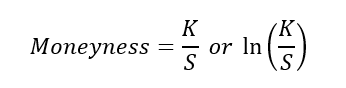
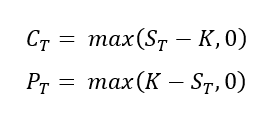
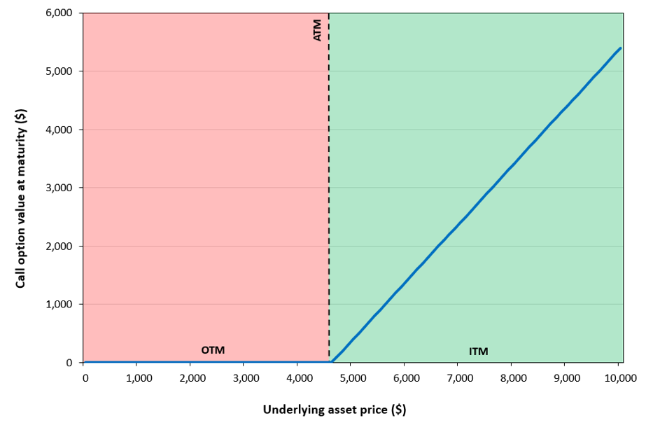
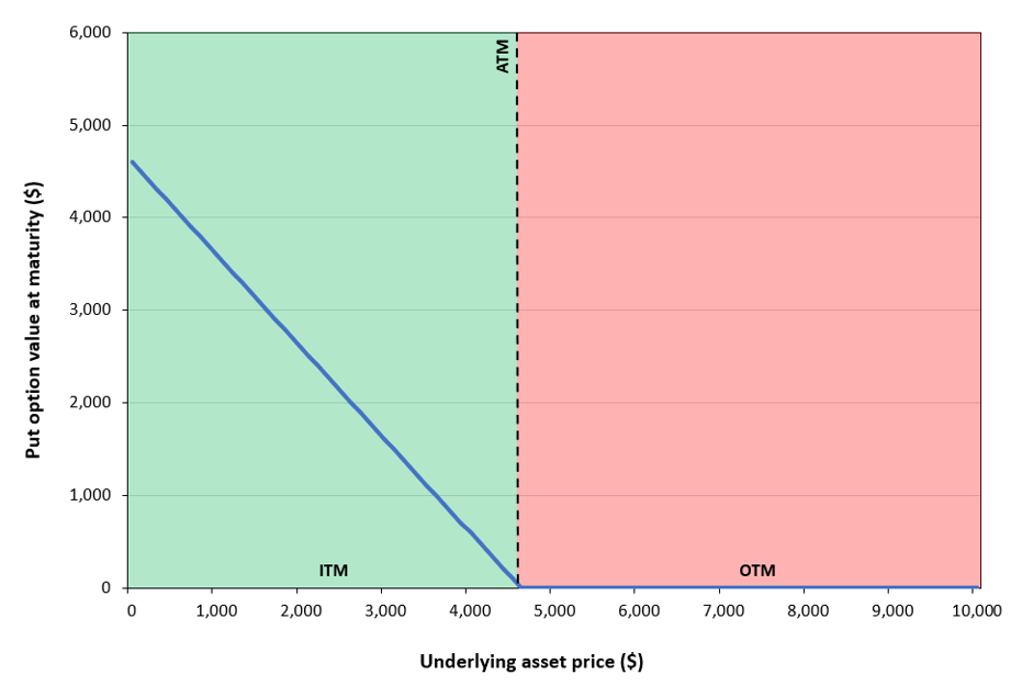
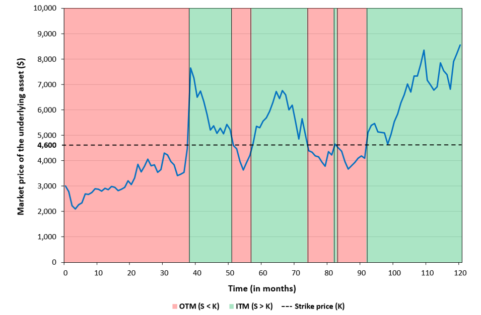
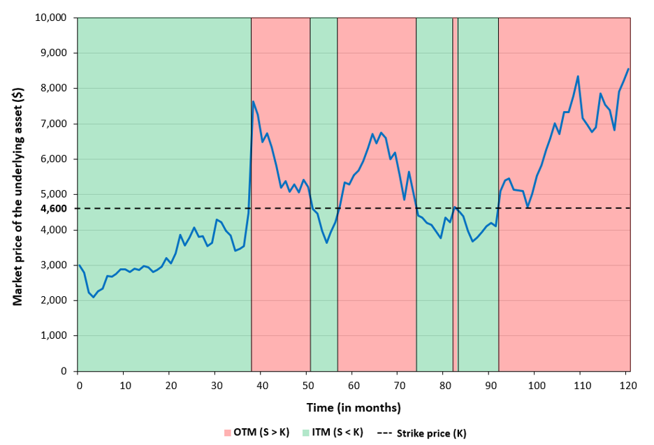
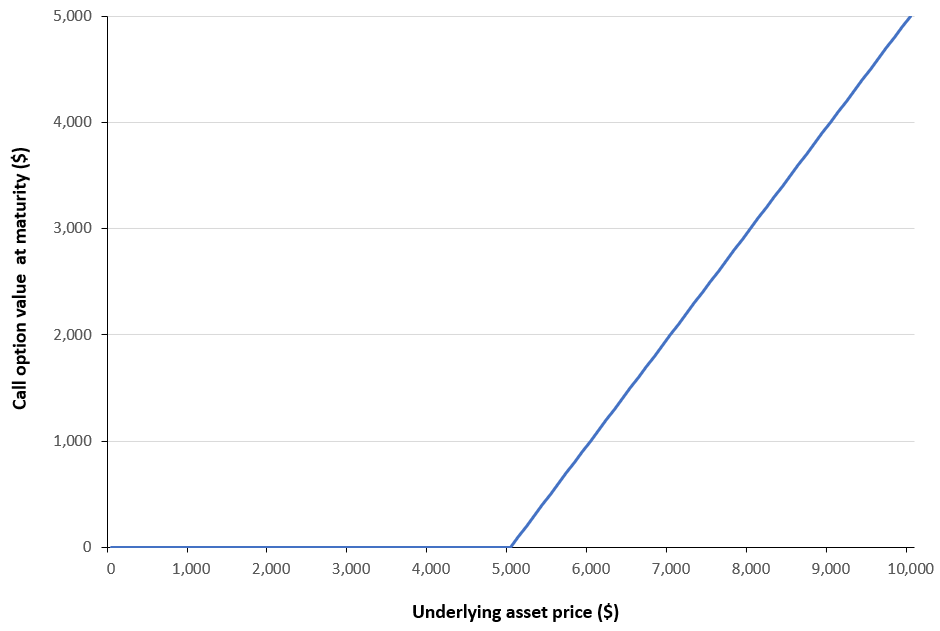
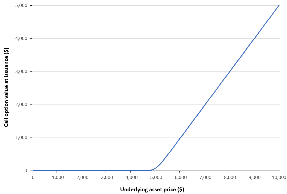
Options are contracts that give the holder the right but not the obligation to buy (call) or sell (put) an asset at a fixed strike price by a given expiration date. The buyer pays an upfront premium to the writer. If the option expires unexercised, the buyer loses only the premium. If exercised, the writer bears the payoff. Options can be American (exercise anytime) or European (exercise only at expiry) and are traded both on exchanges (standardized) and OTC (customized).

Swaps are bilateral contracts to exchange streams of cash flows over time, typically based on fixed versus floating interest rates or other reference indices. Payments are calculated on a notional principal that is not exchanged. Swaps are core OTC instruments for managing interest rate and financial risk.

Types of underlying asset classes

Underlying assets are the products on which a derivative instrument or contract derives its value. The most commonly traded underlying assets are explained below.

Equity derivatives include futures and options on stock indices, such as the S&P 500 Index. These instruments offer capital-efficient ways to manage market risk and enhance returns. Through index futures, institutional investors can achieve cost-effective hedging by locking in prices, while index options provide a non-linear, asymmetric payoff structure that protects against tail risk. Furthermore, equity swaps allow for the seamless exchange of total stock returns for floating interest rates, providing exposure to specific market segments without the capital requirements of direct physical ownership.

Interest rate derivatives include swaps and futures that help manage interest rate risk. Interest rate swaps involve exchanging fixed and floating payments, protecting banks against mismatches between loan income and deposit costs. Interest rate futures allow investors to lock in future borrowing or investment rates and provide insight into market expectations of monetary policy.

Commodity derivatives hedge price risk arising from storage, delivery, and seasonal supply-demand fluctuations. Forwards and futures on crude oil, natural gas, and power are widely used.

Foreign exchange derivatives include forward contracts and cross-currency swaps, allowing firms to hedge currency risk. Cross-currency swaps also support local currency bond markets by enabling hedging of interest and exchange rate risk.

Credit derivatives transfer the risk of default between counterparties. The most widely used is the credit default swap (CDS), which acts like insurance: the buyer pays a premium to receive compensation if a reference entity default.

Quantitative measures of derivatives market activity and size

This section presents the principal measures or statistics used to evaluate the size of the derivatives markets, covering both over-the-counter and exchange-traded instruments, the different derivatives products, and asset classes.

Notional outstanding and gross market value are the primary measures used to assess the size and economic exposure of OTC derivatives markets, while ETDs are typically evaluated using indicators such as open interest and trading volume.

Notional amount

Notional amount, or notional outstanding, is the total principal or reference value of all outstanding derivatives contracts. It captures the overall scale of positions in the derivatives market without reflecting actual market risk or cash exchanged.

For example let us consider a FX forward contract in which two parties agree to exchange $50 for euros in three months at a predetermined exchange rate. The notional amount is $50, because all cash flows (and gains or losses) from the contract are calculated with reference to this amount. No money is exchanged when the contract is initiated, and at maturity only the difference between the agreed exchange rate and the prevailing market rate determines the gain or loss computed on the $50 notional.

Now consider a call option on a stock with a strike price of $50. The notional amount is $50. The option buyer pays only an upfront premium, which is much smaller than $50, but the payoff of the option at maturity depends on how the market price of the stock compares to this $50 reference value.

When measuring notional outstanding in the derivatives market, the notional amounts of all individual contracts are simply added together. For example, one FX forward with a notional of $50 and two option contracts each with a notional of $50 result in a total notional outstanding of $150. This aggregated figure indicates the overall scale of derivatives activity, but it typically overstates actual economic risk because contracts may offset each other and only a fraction of the notional is ever exchanged.

Gross market value

Gross market value is the sum of the absolute values of all outstanding derivatives contracts with either positive or negative replacement (mark-to-market) values, evaluated at market prices prevailing on the reporting date. It reflects the potential scale of market risk and financial risk transfer, showing the economic exposure of a dealer’s derivatives positions in a way that is comparable across markets and products.

To continue the previous FX forward example, suppose a dealer has two outstanding FX forward contracts, each with a notional amount of $50. Due to movements in exchange rates, the first contract has a positive replacement value of $0.50 (the dealer would gain $0.50 if the contract were replaced at current market prices), while the second contract has a negative replacement value of –$0.40. The gross market value is calculated as the sum of the absolute values of these replacement values: |0.50| + |−0.40| = $0.90. Although the total notional outstanding of the two contracts is $100, the gross market value is only $0.90. This measure therefore reflects the dealer’s actual economic exposure to market movements at current prices, rather than the contractual size of the positions.

When this concept is extended to the entire derivatives market, the same distinction becomes apparent at a global scale. While the global derivatives market is often described as having hundreds of trillions of dollars in notional outstanding (approximately USD 850 trillion for OTC derivatives), the economically meaningful exposure is an order of magnitude smaller when measured using gross market value. Unlike notional amounts, gross market value aggregates current mark-to-market exposures, making it a more meaningful and comparable indicator of market risk and financial risk transfer across products and markets.

Open Interest

Open interest refers to the total number of outstanding derivative contracts that have not been closed, expired, or settled. It is calculated by adding the contracts from newly opened trades and subtracting those from closed trades. Open interest serves as an important indicator of market activity and liquidity, particularly in exchange-traded derivatives, as it reflects the level of active positions in the market. Measured at the end of each trading day, open interest is widely used as an indicator of market sentiment and the strength behind price trends.

For example on an exchange, a total of 100 futures contracts on crude oil are opened today. Meanwhile, 30 existing contracts are closed. The open interest at the end of the day would be: 100 (new contracts) − 30 (closed contracts) = 70 contracts. This indicates that 70 contracts remain active in the market, representing the total number of positions that traders are holding.

Trading Volume

Trading volume measures the total number of contracts traded over a specific period, such as daily, monthly, or annually. It provides insight into market liquidity and activity, reflecting how actively derivatives contracts are bought and sold. For OTC markets, trading volume is often estimated through surveys, while for exchange-traded derivatives, it is directly reported.

Consider the same crude oil futures market. If during a single trading day, 50 contracts are bought and 50 contracts are sold (including both new and existing positions), the trading volume for the day would be: 50 + 50 = 100 contracts

Here, trading volume shows how active the market is on that day (flow), while open interest shows how many contracts remain open at the end of the day (stock). High trading volume with low open interest may indicate rapid turnover, whereas high open interest with rising prices can signal strong bullish sentiment.

Key sources of statistics on global derivatives markets

Bank for International Settlements (BIS)

The Bank for International Settlements (BIS) provides quarterly statistics on exchange-traded derivatives (open interest and turnover in contracts, and notional amounts) and semiannual data on OTC derivatives outstanding (notional amounts and gross market values across risk categories like interest rates, FX, equity, commodities, and credit). All the data used in this post has been sourced from the BIS database.

Data are collected from over 80 exchanges for ETDs and via surveys of major dealers in 12 financial centers for OTC derivatives. BIS ensures comparability by standardizing definitions, consolidating country-level data, halving inter-dealer positions to avoid double counting, and converting figures into USD. Interpolations are used to fill gaps between triennial surveys, ensuring consistent time series for analysis.

International Swaps and Derivatives Association (ISDA)

ISDA develops and maintains standardized reference data and contractual frameworks that underpin global OTC derivatives markets. This includes machine-readable definitions and value lists for core market terms such as benchmark rates, floating rate options, currencies, business centers, and calendars, primarily derived from ISDA documentation (notably the ISDA Interest Rate Derivatives Definitions). The data are distributed via the ISDA Library and increasingly designed for automated, straight-through processing.

ISDA’s standards are created and updated through industry working groups and are widely used to support trade documentation, confirmation, clearing, and regulatory reporting. Initiatives such as the Common Domain Model (CDM) and Digital Regulatory Reporting (DRR) translate market conventions and regulatory requirements across multiple jurisdictions into consistent, machine-executable logic. While ISDA does not publish comprehensive market volume statistics, its frameworks play a central role in harmonizing OTC derivatives markets and enabling reliable post-trade transparency.

Futures Industry Association (FIA)

Futures Industry Association (FIA), via FIA Tech, provides comprehensive derivatives data including position limits, exchange fees, contract specifications, and trading volumes for futures/options across global products.

Sources aggregate from exchanges, indices (1,800+ products, 100,000+ constituents), and regulators for reference data like symbologist and corporate actions. The process involves standardizing data into consolidated formats with 500+ attributes, automating regulatory reporting (e.g., CFTC ownership/control), and ensuring compliance via databanks.

How to get the data

The data discussed in this article is drawn from the BIS, FIA and Visual Capitalist. For comprehensive statistics on global derivatives markets (both over-the-counter (OTC) and exchange-traded derivatives (ETDs)), the data are available at https://data.bis.org/ and for exchange-traded derivatives specifically, detailed data are provided by the Futures Industry Association (FIA) through its ETD volume reports, accessible at https://www.fia.org/etd-volume-reports. Data on equity spot market and real economy sectors are sourced from Visual Capitalist.

Derivatives market business statistics

Global derivatives market

In this section, we focus on two core measures of derivatives market activity and size: the notional amount outstanding and the gross market value, which together provide complementary perspectives on the scale of contracts and the associated economic exposure.

As of 30^th July 2025, the global derivatives market is estimated to have an outstanding notional value of approximately USD 964 trillion, according to the Bank for International Settlements (BIS). As illustrated in the figure below, the market is largely dominated by over-the-counter (OTC) derivatives, which account for nearly 88% of total notional amounts, whereas exchange-traded derivatives (ETDs) represent a comparatively smaller share of about USD 118 trillion.

Figure 1. Derivatives Markets: OTC versus ETD (2025)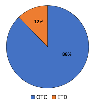
Derivatives Markets: OTC and ETD (2025)
Source: computation by the author (BIS data of 2025).

Figure 2 below compares the scale of the global equity derivatives market with that of the underlying equity spot market as of mid-2025. The figure shows that, although equity derivatives represent a sizeable market in notional terms, they are still much smaller than the equity spot market measured by market capitalization. This suggests that the primary locus of economic value in equities remains in the spot market, while the derivatives market mainly represents contingent claims written on that underlying value rather than a comparable pool of market wealth. The relatively small gross market value of equity derivatives further indicates that only a limited portion of derivative notional translates into actual market exposure.

Figure 2. Equity Markets: Spot versus Derivatives (2025)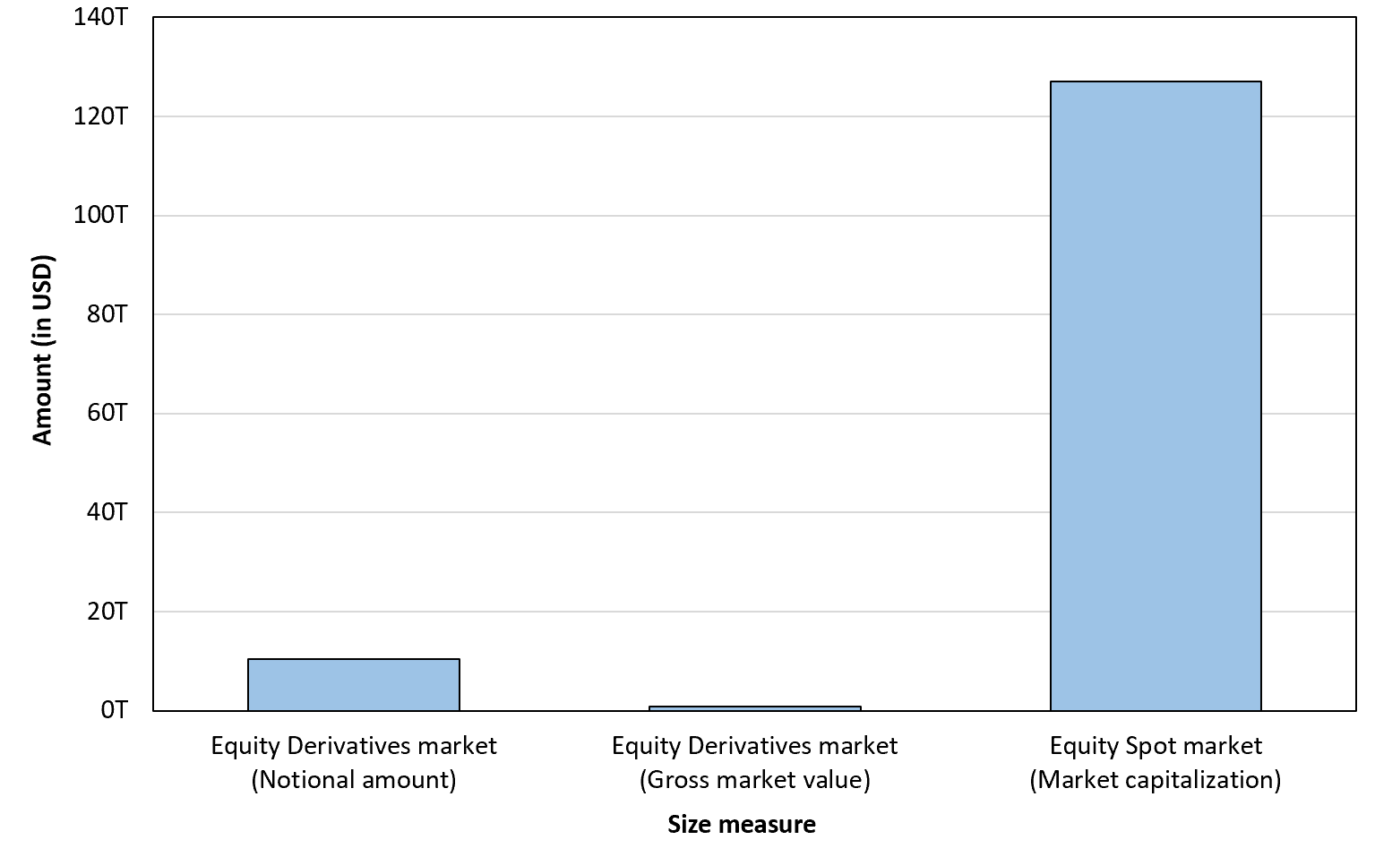

Source: computation by the author (BIS and Visual Capitalist data of 2025).

Data sources: global derivatives notional outstanding as of mid-2025 BIS OTC and exchange traded data; global equity spot market capitalization as of 2025 (Visual Capitalist).

Figure 3 below juxtaposes the global derivatives market with selected real-economy sectors to provide an intuitive comparison of scale. Values are reported in USD trillions and plotted on a logarithmic axis, such that equal distances along the horizontal scale correspond to ten-fold (×10) changes in magnitude rather than linear increments. This representation allows quantities that differ by several orders of magnitude to be meaningfully displayed within a single chart.

Interpreted in this manner, the figure illustrates that the notional size of derivatives markets far exceeds the market capitalization of major real-economy sectors, including technology, financials, energy, fast moving consumer goods (FMCG), and luxury. The comparison is illustrative rather than like-for-like, and is intended to contextualize the scale of financial contract exposure rather than to imply equivalent economic value or direct risk.

Figure 3. Scale of Global Derivatives Relative to Major Real-Economy Sectors (2025)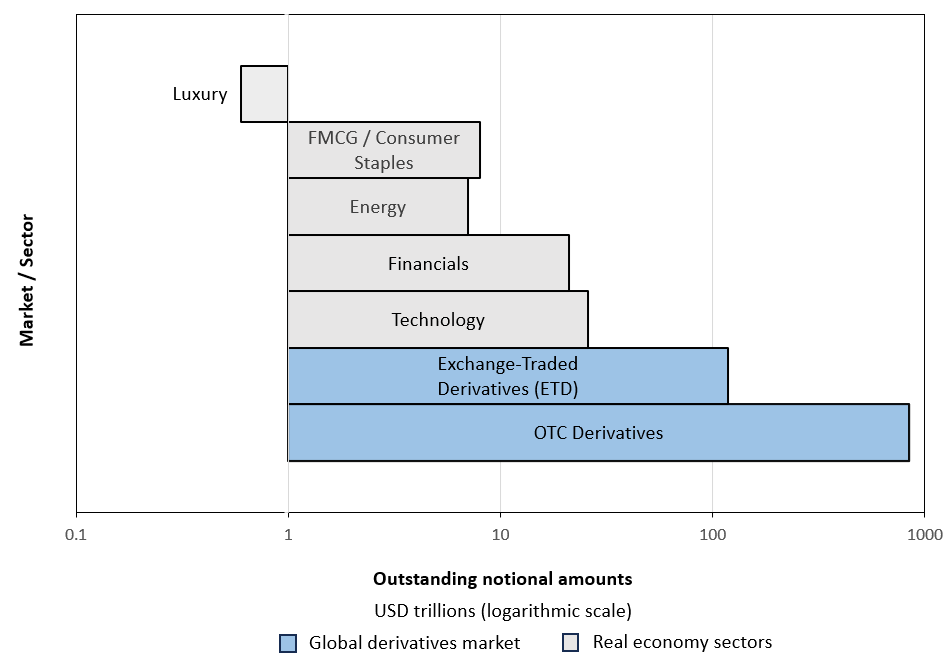

Source: computation by the author (BIS and Visual Capitalist data).

Data sources: BIS OTC derivatives statistics (June 2025) for notional outstanding; Visual Capitalist global stock market sector data (2025) for sector market capitalizations; companies market cap / Visual Capitalist for luxury company market caps.

OTC derivatives market

Figures 4 and 5 below illustrate the evolution of the OTC derivatives market from 1998 to 2025 using the two measures discussed above: outstanding notional amounts (Figure 4) and gross market value (Figure 5). As the data show, notional outstanding tends to overstate the effective economic size of the market, as it reflects contractual face values rather than actual risk exposure. By contrast, gross market value provides a more economically meaningful measure by capturing the current cost of replacing outstanding contracts at prevailing market prices.

Figure 4. Size of the OTC Derivatives Market (Notional amount)
Size of the OTC derivative market (Notional amount)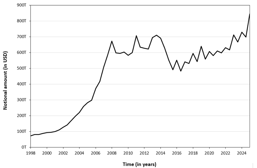
Source: computation by the author (BIS data).

Figure 5. Size of the OTC Derivatives Market (Gross market value)
Size of the OTC derivative market (Gross market value)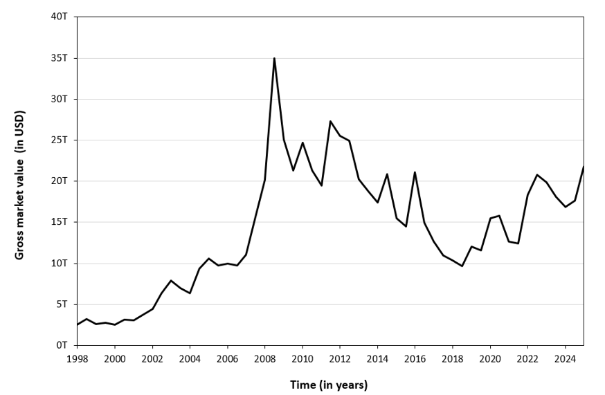
Source: computation by the author (BIS data).

The figure below illustrates the OTC derivatives market data as of 30^th July 2025 based on the two metrics discussed above: outstanding notional amounts and gross market value. As the data show, Gross market value (GMV) represents only about 2.6% of total notional outstanding, highlighting the large gap between contractual face values and economically meaningful exposure.

Figure 6. Size measure of the OTC derivatives market (2025)
Size of the OTC derivative market (2025)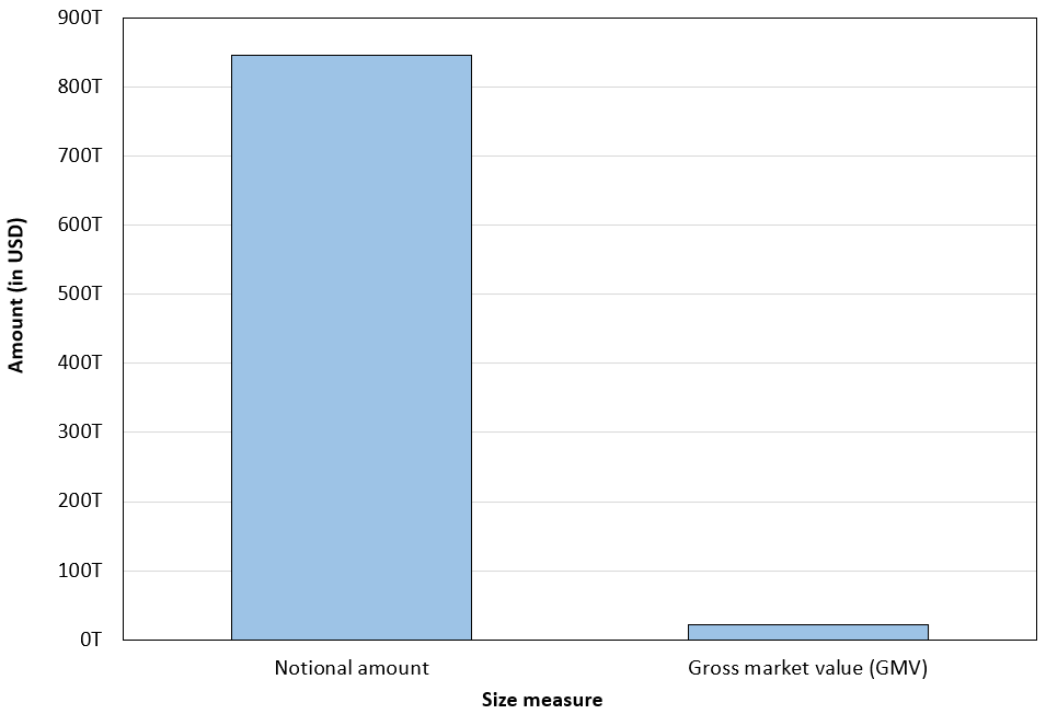
Source: computation by the author (BIS data).

Exchange-traded derivatives market

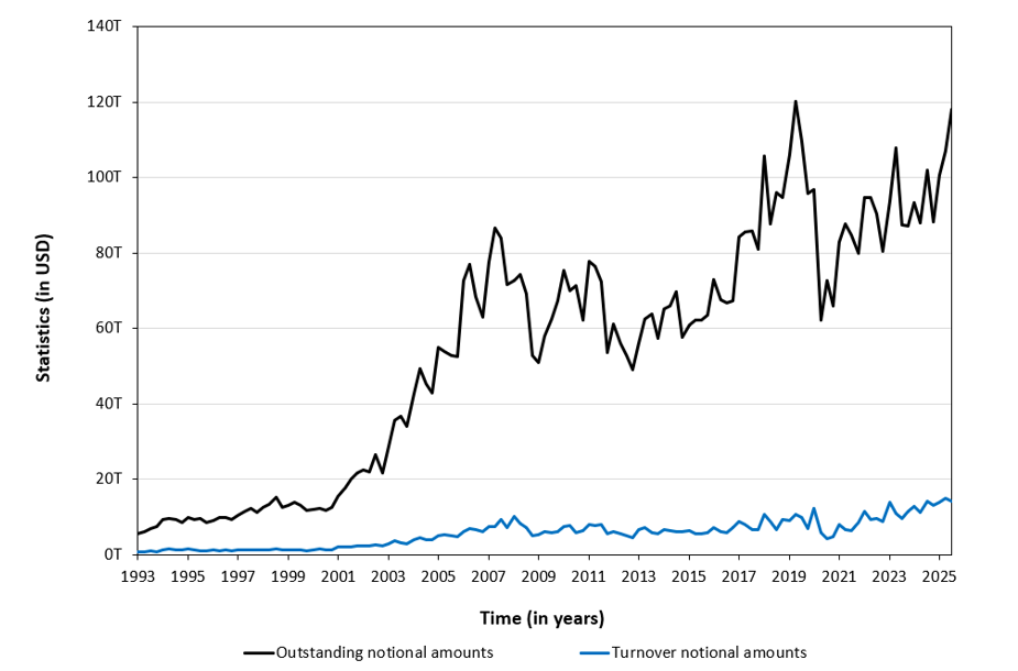
Figure 7 below illustrates the growth of the exchange-traded derivatives market from 1993 to 2025, based on outstanding notional amounts (open interest) and turnover notional amounts (trading volume). For comparability across contracts and exchanges, open interest is expressed in notional terms by multiplying the number of open contracts by their contract size, yielding US dollar equivalents. Turnover is defined as the notional value of all futures and options traded during the period, with each trade counted once.

Figure 7. Size of the Exchange-Traded Derivatives Market
Size of the exchange traded derivatives market
Source: computation by the author (BIS data).

The figure below illustrates the exchange-traded derivatives market data as of 30^th July 2025 based on the two metrics discussed above: open interest and turnover (trading volume). The chart shows that only about 12%, of the open positions is actively traded, highlighting the difference between market size and the trading activity.

Figure 8. Size of the Exchange traded derivatives market (2025)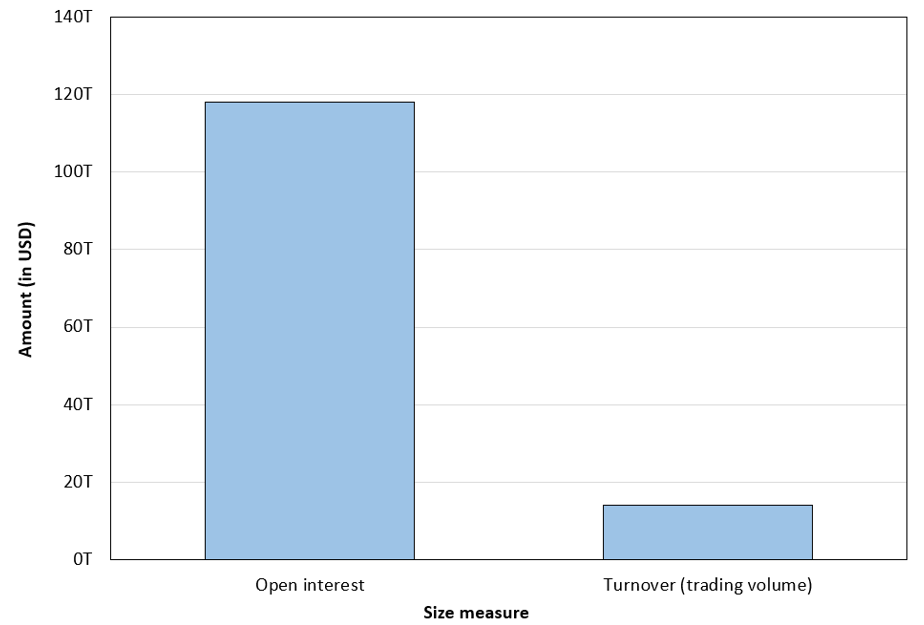

Source: computation by the author (BIS data).

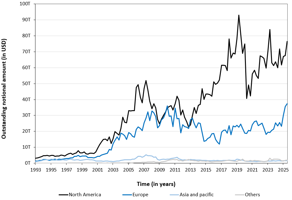
Figure 9 below illustrates the evolution of the global exchange-traded derivatives market from 1993 to 2025, measured by outstanding notional amounts across major regions. The figure reveals a pronounced concentration of activity in North America and Europe, which drives most of the market’s expansion over time, while Asia-Pacific and other regions play a more modest role. Despite cyclical fluctuations, the overall trajectory is one of sustained long-run growth, underscoring the increasing importance of exchange-traded derivatives in global risk management and price discovery.

Figure 9. Size of the Exchange-Traded Derivatives Market by geographical locations
Size of the exchange traded derivatives market by geographic location
Source: computation by the author (BIS data).

Underlying asset classes

This section analyzes underlying asset-class statistics for derivatives traded in exchange-traded (ETD) and over-the-counter (OTC) markets.

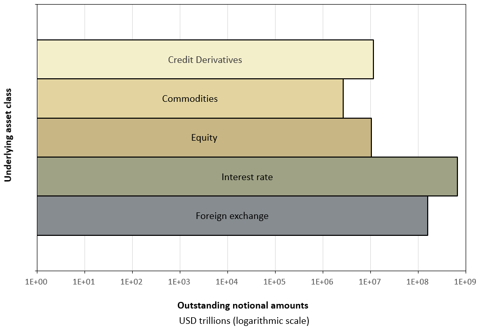
Figure 10 below presents the distribution of exchange-traded derivatives (ETDs) activity across major underlying asset classes. When measured by the number of contracts traded (volume), the market is highly concentrated, with Equity derivatives dominating and accounting for the vast majority of activity. This is followed at a significant distance by Interest Rate and Commodity derivatives. However, this distribution reverses when measured by the notional value of outstanding contracts, where Interest Rate derivatives represent the largest share of the market due to the high underlying value of each contract.

Figure 10. Size of the exchange-traded derivatives market by asset classes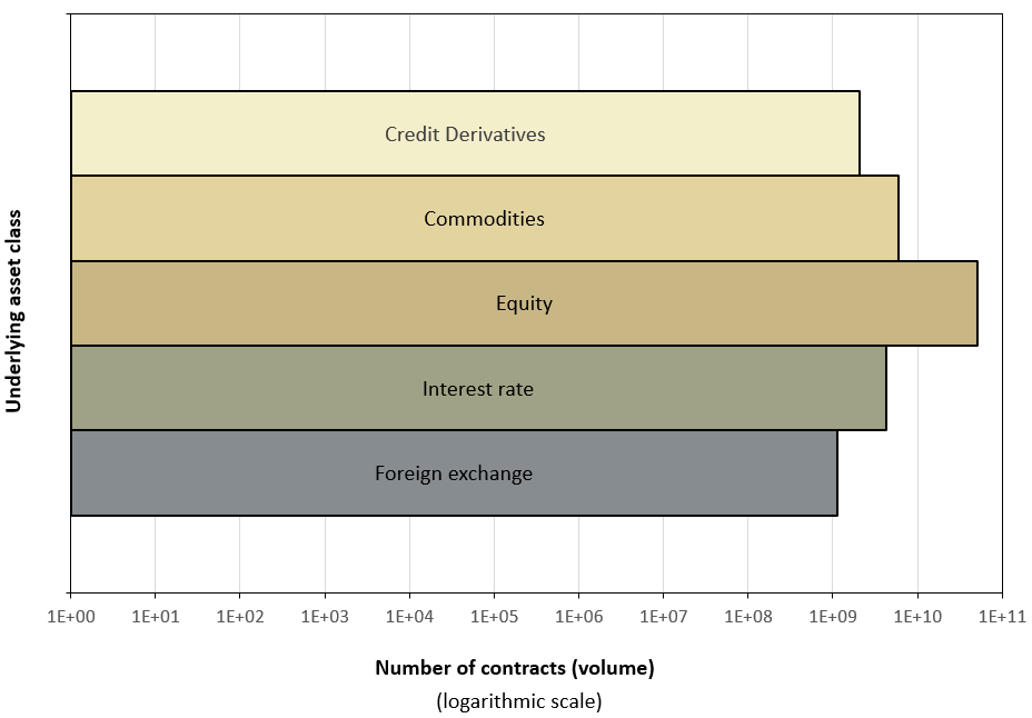
Size of the exchange traded derivatives market
Source: computation by the author (FIA data).

Figure 11 below presents the distribution of OTC derivatives activity across major underlying asset classes, measured by the outstanding notional amounts and displayed on a logarithmic scale. Read in this way, the chart shows that OTC activity is broadly diversified across interest rates, equity indices, commodities, foreign exchange, and credit, with interest rate and foreign exchange derivatives accounting for the largest contract volumes.

Figure 11. Size of the OTC derivatives market by asset classes
Size of the exchange traded derivatives market
Source: computation by the author (BIS data).

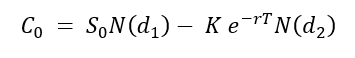
Role of the Black–Scholes–Merton (BSM) model

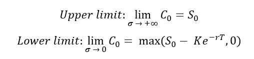
The Black–Scholes–Merton (BSM) model played a role in financial markets that extended well beyond option pricing. As argued by MacKenzie and Millo (2003), once adopted by traders and exchanges, it actively shaped how options markets were organized, priced, and operated rather than merely describing pre-existing price behaviour. Its use at the Chicago Board Options Exchange (CBOE) helped standardize quoting practices, enabled model-based hedging, and supported the rapid growth of liquidity in listed options markets.

At a broader level, MacKenzie (2006) shows that BSM contributed to a transformation in financial culture by embedding theoretical assumptions about risk, volatility, and rational pricing into everyday market practice. In this sense, BSM acted as an “engine” that reshaped markets and economic behaviour, not simply a “camera” recording them.

Beyond markets and firms, the diffusion of the BSM model also had wider societal implications. By formalizing risk as something that could be quantified, priced, and hedged, BSM contributed to a broader cultural shift in how uncertainty was perceived and managed in modern economies (MacKenzie, 2006). This reframing reinforced the view that complex economic risks could be controlled through mathematical models, with public perceptions of financial stability.

Why should you be interested in this post?

For anyone aiming for a career in finance, understanding the derivatives market is essential, as it is currently one of the most actively traded markets and is expected to grow further. Studying the statistics and business impact of derivatives provides valuable context on past challenges and the solutions developed to manage risks, offering a solid foundation for analyzing and navigating modern financial markets.

Useful resources

Academic research on option pricing

Black F. and M. Scholes (1973) The pricing of options and corporate liabilities. Journal of Political Economy, 81(3), 637–654.

Merton R.C. (1973) Theory of rational option pricing. The Bell Journal of Economics and Management Science, 4(1), 141–183.

Hull J.C. (2022) Options, Futures, and Other Derivatives, 11th Global Edition, Chapter 15 – The Black–Scholes–Merton model, 338–365.

Academic research on the role of models

MacKenzie, D., & Millo, Y. (2003). Constructing a Market, Performing Theory: The Historical Sociology of a Financial Derivatives Exchange. American Journal of Sociology, 109(1), 107–145.

MacKenzie, D. (2006). An Engine, not a Camera: How Financial Models Shape Markets. MIT Press.

Data

Bank for International Settlements (BIS). Retrieved from BIS Statistics Explorer.

Futures Industry Association (FIA). Retrieved from ETD Volume Reports.

Visual Capitalist. Retrieved from The Global Stock Market by Sector.

Visual Capitalist. Retrieved from Piecing Together the $127 Trillion Global Stock Market.

About the author

The article was written in February 2026 by Saral BINDAL (Indian Institute of Technology Kharagpur, Metallurgical and Materials Engineering, 2024-2028 & Research assistant at ESSEC Business School).

▶ Discover all articles written by Saral BINDAL

Volatility curves: smiles and smirks

January 31, 2026January 31, 2026 by Saral BINDAL

In this article, Saral BINDAL (Indian Institute of Technology Kharagpur, Metallurgical and Materials Engineering, 2024-2028 & Research assistant at ESSEC Business School) analyzes the various shapes of volatility curves observed in financial markets and explains how they reveal market participants’ beliefs about future asset price distributions as implied by option prices.

Introduction

In financial markets characterized by uncertainty, volatility is a fundamental factor shaping the dynamics of the prices of financial instruments. Implied volatility stands out as a key metric as a forward-looking measure that captures the market’s expectations of future price fluctuations, as reflected in current market prices of options.

Implied volatility is inherently a two-dimensional object, as it is indexed by strike K and maturity T. The collection of these implied volatilities across all strikes and maturities constitutes the volatility surface. Under the Black–Scholes–Merton (BSM) framework, volatility is assumed to be constant across strikes and maturities, in which case the volatility surface would degenerate into a flat plane. Empirically, however, the volatility surface is highly structured and varies significantly across both strike and maturity.

Accordingly, this post focuses on implied volatility curves across moneyness for a fixed maturity (i.e. cross-sections of the volatility surface), examining their canonical shapes, economic interpretation, and the insights they reveal about market beliefs and risk preferences.

Option pricing

Option pricing aims to determine the fair value of options (calls and puts). One of the most widely used frameworks for this purpose is the Black–Scholes–Merton (BSM) model, which expresses the option value as a function of five key inputs: the underlying asset price S, the strike price K, time to maturity T, the risk-free interest rate r, and volatility σ. Given these parameters, the model yields the theoretical value of the option under specific market assumptions. The details of the BSM option pricing formulas along with variable definitions can be found in the article Black-Scholes-Merton option pricing model.

Implied volatility

In the Black–Scholes–Merton (BSM) model, volatility is an unobservable parameter, representing the expected future variability of the underlying asset over the option’s remaining life. In practice, implied volatility is obtained by inverting the BSM pricing formula (using numerical methods such as the Newton–Raphson algorithm) to find the specific volatility that equates the BSM theoretical price to the observed market price. The details for the mathematical process of calculation of implied volatility can be found in Implied Volatility and Option Prices.

Moneyness

Moneyness describes the relative position of an option’s strike price K with respect to the current underlying asset price S. It indicates whether the option would have a positive intrinsic value if exercised at the current moment. Moneyness is typically parameterized using ratios such as K/S or its logarithmic transform.

Moneyness formula

In practice, moneyness classifies an option based on its intrinsic value. An option is said to be in-the-money (ITM) if it has positive intrinsic value, at-the-money (ATM) if its intrinsic value is zero, and out-of-the-money (OTM) if its intrinsic value is zero and immediate exercise would not be optimal. In terms of the relationship between the underlying asset price (S) and the strike price (K), a call option is ITM when S > K, ATM when S = K, and OTM when S < K. Conversely, a put option is ITM when S < K, ATM when S = K, and OTM when S > K.

The payoff, that is the cash flow realized upon exercising the option at maturity T, is given for call and put options by:

Payoff formula for call and put options

where S_T is the underlying asset price at the time the option is exercised.

Figure 1 below illustrates the payoff of a call option, that is the call option value at maturity as a function of its underlying asset price. The call option’s strike price is assumed to be equal to $4,600. For an underlying price of $3,000, the call option is out-of-the-money (OTM); for a price of $4,600, the call option is at-the-money (ATM); and for a price of $7,000, the call option is in-the-money (ITM) and worth $2,400.

Figure 1. Payoff for a call option and its moneyness (OTM, ATM and ITM)

Source: computation by the author.

Similarly, Figure 2 below illustrates the payoff of a put option, that is the put option value at maturity as a function of its underlying asset price. The put option’s strike price is assumed to be equal to $4,600. For an underlying price of $3,000, the put option is in-the-money (ITM) and worth $1,600; for a price of $4,600, the put option is at-the-money (ATM); and for a price of $7,000, the put option is out-of-the-money (OTM).

Figure 2. Payoff for a put option and its moneyness (OTM, ATM and ITM)

Source: computation by the author.

Figure 3 below illustrates the temporal dynamics of moneyness for a European call option with a strike price of $4,600, showing how the option transitions between out-of-the-money, at-the-money, and in-the-money states as the underlying asset price moves relative to the strike over its lifetime.

Figure 3. Evolution of a call option moneyness

Source: computation by the author.

Similarly, Figure 4 below illustrates the temporal dynamics of moneyness for a European put option with a strike price of $4,600, showing how the option transitions between out-of-the-money, at-the-money, and in-the-money states as the underlying asset price moves relative to the strike over its lifetime.

Figure 4. Evolution of a put option moneyness

Source: computation by the author.

You can download the Excel file below for the computation of moneyness of call and put options as discussed in the above figures.

Empirical observation: implied volatility depends on moneyness

Smiles and smirks

Volatility curves refer to plots of implied volatility across different strikes for options with the same maturity. Two distinct shapes are commonly observed: the “volatility smile” and the “volatility smirk”.

A volatility smile is a symmetric pattern commonly observed in options markets. For a given underlying asset and expiration date, it is defined as the mapping of option strike prices to their Black–Scholes–Merton implied volatilities. The term “smile” refers to the distinctive shape of the curve: implied volatility is lowest near the at-the-money (ATM) strike and rises for both lower in-the-money (ITM) strikes and higher out-of-the-money (OTM) strikes.

A volatility smirk (also called skew) is an asymmetric pattern in the implied volatility curve and is mainly observed in the equity markets. It is characterized by high implied volatilities at lower strikes and progressively lower implied volatilities as the strike increases, resulting in a downward-sloping profile. This shape reflects the uneven distribution of implied volatility across strikes and stands in contrast to the more symmetric volatility smile observed in other markets.

Stylized facts about the implied volatility curve across markets

Stylized facts characterizing implied volatility curves are persistent and statistically robust empirical regularities observed across financial markets. Below, I discuss the key stylized facts for major asset classes, including equities, foreign exchange, interest rates, commodities, and cryptocurrencies.

Equity market: For major equity indices, the implied volatility curve at a given maturity is typically a negatively sloped smirk: IV is highest for out of the money puts and declines as the strike moves up, rather than forming a symmetric smile (Zhang & Xiang, 2008). This left skew is persistent across maturities and provides useful signals at the individual stock level, where steeper smirks (higher OTM put vs ATM IV) forecast lower subsequent returns, consistent with markets pricing crash risk into downside options (Xing, Zhang & Zhao, 2010).

FX market: For foreign currency options, implied volatility curves most often display a U shaped smile: IV is lowest near at the money and higher for deep in or out of the money strikes, especially for major FX pairs (Daglish, Hull & Suo, 2007). The degree of symmetry depends on the correlation between the FX rate and its volatility, so near zero correlation gives a roughly symmetric smile, while non zero correlations generate skews or smirks that have been empirically documented in options on EUR/USD, GBP/USD and AUD/USD (Choi, 2021).

Commodity market: For commodity options, cross market evidence shows that implied volatility curves are generally negatively skewed with positive curvature, meaning they exhibit smirks rather than flat surfaces, with higher IV for downside strikes but still some smile like curvature (Jia, 2021). Studies on crude oil and related commodities also find pronounced smiles and smirks whose strength varies with fundamentals such as inventories and hedging pressure, reinforcing it is a core stylized fact in commodity derivatives (Soini, 2018; Vasseng & Tangen, 2018).

Fixed income market: Swaption markets display smiles and skews on their volatility curves: for a given expiry and tenor, implied volatility typically curves in moneyness and may tilt up or down depending on the correlation between the underlying rate and volatility (Daglish, Hull & Suo, 2007). Empirical work on the swaption volatility cube shows that simple one factor or SABR lifted constructions do not capture the full observed smile, indicating that a rich, strike and maturity dependent IV surface is itself a stylized feature of interest rate options (Samuelsson, 2021).

Crypto market: Bitcoin options exhibit a non flat implied volatility smile with a forward skew, and short dated options can reach very high levels of implied volatility, reflecting heavy tails and strong demand for certain strikes (Zulfiqar & Gulzar, 2021). Because of this forward skew, the paper concludes that Bitcoin options “belong to the commodity class of assets,” although later studies show that the Bitcoin smile can change shape across regimes and is often flatter than equity index skew (Alexander, Kapraun & Korovilas, 2023).

Summary of stylized facts about implied volatility

An Empirical Analysis of S&P 500 Implied Volatility

This section describes the data, methodology, and empirical considerations for the analysis of implied volatility of put options written on the S&P 500 index. We begin by highlighting a classical challenge in cross-sectional option data: asynchronous trading.

Asynchronous trading and measurement error

In empirical option pricing, the non-synchronous observation of option prices and the underlying asset price generates measurement errors in implied volatility estimation, as the building of the volatility curve based on an option pricing model relies on option prices with the underlying price observed at the same point of time.

Formally, let the option price C be observed at time t_c, while the underlying asset price S is observed at time t_s with t_s ≠ t_c. The observed option price therefore satisfies

Asynchronous call option price and underlying asset price

Since the option price at time t_c depends on the latent spot price S(t_c), rather than the asynchronously observed price S(t_s), this mismatch introduces measurement error in the underlying price variable and implied volatility at the end.

Various standard filters including no-arbitrage, liquidity, moneyness, maturity, and implied-volatility sanity checks are typically applied to mitigate errors-in-variables arising from asynchronous observations of option prices and their underlying assets.

Example: options on the S&P 500 index

Consider the following sample of option data written on the S&P 500 index. Data can be obtained from FirstRate Data.

Figure 5 below illustrates the volatility smirk (or skew) for an option chain (a series of option prices for the same maturity) written on the S&P 500 index traded on 3rd July 2023 with time to maturity of 2 days after filtering it out from the above data.

Figure 5. Volatility smirk for put option prices on the S&P 500 index
Volatility smirk computed for put option on the S&P 500 index
Source: computation by the author.

You can download the Excel file below to compute the volatility curve for put options on the S&P 500 index.

Economic Insights

This section explains how the shape of the implied volatility curve reveals key economic forces in options markets, including demand for crash protection, leverage-driven volatility feedback effects, and the role of market frictions and limits to arbitrage.

Demand for crash protection:

Out-of-the-money put options serve as insurance against market crashes and hedge tail risk. Because this demand is persistent and largely one-sided, put options become expensive relative to their Black–Scholes-Merton values, resulting in elevated implied volatilities at low strikes. This excess pricing reflects the market’s willingness to pay a premium to insure against rare but severe losses.

Leverage and volatility feedback effects:

When equity prices fall, firms become more leveraged because the value of equity declines relative to debt. Higher leverage makes equity riskier, increasing expected future volatility. Anticipating this effect, markets assign higher implied volatility to downside scenarios than to upside moves. This endogenous feedback between price declines, leverage, and volatility naturally produces a negative volatility skew, even in the absence of crash-risk preferences.

Market frictions and limits to arbitrage:

In practice, option writers are subject to capital constraints, margin requirements, and exposure to jump and tail risk. These constraints limit their capacity to supply downside protection at low prices. As a result, downside options embed not only compensation for fundamental crash risk, but also a risk premium reflecting the balance-sheet costs and risk-bearing capacity of intermediaries. The observed volatility skew therefore arises endogenously from limits to arbitrage rather than purely from differences in underlying return distributions.

Conclusion

The dependence of implied volatility on moneyness is neither an anomaly nor a technical artifact. It reflects market expectations, risk preferences, and the perceived probability of extreme outcomes. For both pedagogical and investment applications, the implied volatility curve is a central tool for understanding how markets price tail and downside risk.

Why should I be interested in this post?

Understanding implied volatility and its relationship with moneyness extends beyond option pricing, offering insights into how markets perceive risk and assess the likelihood of extreme events. Patterns such as volatility smiles and skews reflect investor behavior, the demand for protection, and the asymmetric emphasis on potential losses over gains, providing a clearer view of both pricing anomalies and the economic forces that shape financial markets.

Useful resources

Academic research on Option pricing

Black, F., & Scholes, M. (1973). The pricing of options and corporate liabilities, Journal of Political Economy, 81(3), 637–654.

Hull J.C. (2015) Options, Futures, and Other Derivatives, Ninth Edition, Chapter 15 – The Black-Scholes-Merton model, 343-375.

Merton, R.C. (1973). Theory of rational option pricing, The Bell Journal of Economics and Management Science, 4(1), 141–183.

Academic research on Stylized facts

Alexander, C., Kapraun, J. & Korovilas, D. (2023) Delta hedging bitcoin options with a smile, Quantitative Finance, 23(5), 799–817.

Bakshi, G., Cao, C., & Chen, Z. (1997). Empirical performance of alternative option pricing models, The Journal of Finance, 52(5), 2003–2049.

Bates, D. S. (1991). The crash of ’87: Was it expected? The evidence from options markets, The Journal of Finance, 46(5), 1777–1819.

Bates, D. S. (2000). Post-’87 crash fears in the S&P 500 futures option market, Journal of Econometrics, 94(1–2), 181–238.

Choi, K. (2021) Foreign exchange rate volatility smiles and smirks, Applied Stochastic Models in Business and Industry, 37(3), 405–425.

Daglish, T., Hull, J. & Suo, W. (2007) Volatility surfaces: theory, rules of thumb, and empirical evidence, Quantitative Finance, 7(5), 507–524.

Jia, G. (2021) The implied volatility smirk of commodity options, Journal of Futures Markets, 41(1), 72–104.

Samuelsson, A. (2021) Empirical study of methods to complete the swaption volatility cube. Master’s thesis, Uppsala University.

Soini, E. (2018) Determinants of volatility smile: The case of crude oil options. Master’s thesis, University of Vaasa.

Xing, Y., Zhang, X. & Zhao, R. (2010) What does individual option volatility smirk tell us about future equity returns? Review of Financial Studies, 23(5), 1979–2017.

Zhang, J.E. & Xiang, Y. (2008) The implied volatility smirk, Quantitative Finance, 8(3), 263–284.

Zulfiqar, N. & Gulzar, S. (2021) Implied volatility estimation of bitcoin options and the stylized facts of option pricing, Financial Innovation, 7(1), 67.

About the author

The article was written in January 2026 by Saral BINDAL (Indian Institute of Technology Kharagpur, Metallurgical and Materials Engineering, 2024-2028 & Research assistant at ESSEC Business School).

▶ Discover all articles written by Saral BINDAL

Modeling Asset Prices in Financial Markets: Arithmetic and Geometric Brownian Motions

January 30, 2026January 10, 2026 by Saral BINDAL

In this article, Saral BINDAL (Indian Institute of Technology Kharagpur, Metallurgical and Materials Engineering, 2024-2028 & Research assistant at ESSEC Business School) presents two statistical models used in finance to describe the time behavior of asset prices: the arithmetic Brownian motion (ABM) and the geometric Brownian motion (GBM).

Introduction

In financial markets, performance over time is governed by three fundamental variables: the drift (μ), volatility (σ), and maybe most importantly time (T). The drift represents the expected growth rate of the price and corresponds to the expected return of assets or portfolios. Volatility measures the uncertainty or risk associated with price fluctuations around this expected growth and corresponds to the standard deviation of returns. The relationship between these variables reflects the trade-off between risk and return. Time, which is related to the investment horizon set by the investor, determines how both performance and risk accumulate. Together, these variables form the foundation of asset pricing to model the behavior of market price over time, and in fine the performance of the investor at their investment horizon.

Modeling asset prices

Asset price modeling is used to understand the expected return and risk in asset management, risk management, and the pricing of complex financial products such as options and structured products. Although asset prices are influenced by countless unpredictable risk factors, quants in finance always try to find a parsimonious way to model asset prices (using a few parameters only).

The first study of asset price modelling dates from Louis Bachelier in 1900, in his doctoral thesis Théorie de la Spéculation (The Theory of Speculation), where he modelled stock prices as a random walk and applied this framework to option valuation. Later, in 1923, the mathematician Norbert Wiener formalized these ideas as the Wiener process, providing the rigorous stochastic foundation that underpins modern finance.

In the 1960s, Paul Samuelson refined Bachelier’s model by introducing the geometric Brownian motion, which ensures positive stock prices following a lognormal statistical distribution. His 1965 paper “Rational Theory of Warrant Pricing” laid the groundwork for modern asset price modelling, showing that discounted stock prices follow a martingale.

We detail below the two models usually used in finance to model the evolution of asset prices over time: the arithmetic Brownian motion (ABM) and the geometric Brownian motion (GBM). We will then use these models to simulate the evolution of asset prices over time with the Monte Carlo simulation method.

Arithmetic Brownian motion (ABM)

Theory

One of the most widely used stochastic processes in financial modeling is the arithmetic Brownian motion, also known as the Wiener process. It is a continuous stochastic process with normally distributed increments. Using the Wiener process notation, an asset price model in continuous time based on an ABM can be expressed as the following stochastic differential equation (SDE):

SDE for the arithmetic Brownian motion

where:

dS_t = infinitesimal change in asset price at time t t
μ = drift (growth rate of the asset price)
σ = volatility (standard deviation)
dW_t = infinitesimal increment of wiener process (N(0,dt))

Note that the standard Brownian motion is a special case of the arithmetic Brownian motion with a mean equal to zero and a variance equal to one.

In this model, both μ and σ are assumed to be constant over time. It can be shown that the probability distribution function of the future price is a normal distribution implying a strictly positive (although negligible in most cases) probability for the price to be negative.

Integrating the SDE for dS_t over a finite interval (from time 0 to time t), we get:

Integrated SDE for the arithmetic Brownian motion

Here, W_t is defined as W_t = √t · Z_t, where Z_t is a normal random variable drawn from the standard distribution N(0, 1) with mean equal to 0 and variance equal to 1.

At any date t, we can also compute the expected value and a confidence interval such that the asset price S_t lies between the lower and upper bound of the interval with probability equal to 1-α.

Theoritical formulas for mean, upper and lower limits of ABM model

Where S₀ is the initial asset price and z_α.

The z-score for a confidence level of (1 – α) can be calculated as:

z-score formula

where Φ^-1 denotes the inverse cumulative distribution function (CDF) of the standard normal distribution.

For example the statistical z-score (z_α) values for 66%, 95%, and 99% confidence intervals are as the following:

z-score examples

Monte Carlo simulations with ABM

Since Monte Carlo simulations are performed in discrete time, the underlying continuous-time asset price process (ABM) is approximated using the Euler–Maruyama discretization of SDEs (see Maruyama, 1955), as shown below.

Discretization formula for the arithmetic Brownian motion (ABM)

where Δt denotes the time step, expressed in the same time units as the drift parameter μ and the volatility parameter σ (usually the annual unit). For example, Δt may be equal to one day (=1/252) or one month (=1/12).

Figure 1 below illustrates a single simulated asset price path under an arithmetic Brownian motion (ABM), sampled at monthly intervals (Δt = 1/12) over a 10-year horizon (T = 10). Alongside the simulated path, the figure shows the expected (mean) price trajectory and the corresponding upper and lower bounds of a 66% confidence interval. In this example, the model assumes an annual drift (μ) of $8, representing the expected growth rate, and an annual volatility (σ) of $15, capturing random price fluctuations. The initial asset price (S₀) is equal to $100.

Figure 1. Single Monte Carlo–simulated asset price path under an Arithmetic Brownian Motion model.
A Monte Carlo–simulated price path under an arithmetic Brownian motion model
Source: computation by the author (with Excel).

Figure 2 below illustrates 1,000 simulated asset price paths generated under an arithmetic Brownian motion (ABM). In addition to the simulated paths, the figure displays the expected (mean) price trajectory along with the corresponding upper and lower bounds of a 66% confidence interval, using the same parameter settings as in Figure 1.

Figure 2. Monte Carlo–simulated asset price paths under an Arithmetic Brownian Motion model.
Monte Carlo–simulated price paths under an arithmetic Brownian motion model.
Source: computation by the author (with R).

Geometric Brownian motion (GBM)

Theory

Since an arithmetic Brownian motion (ABM) can take negative values, it is unsuitable for directly modeling stock prices if we assume limited liability for investors. Under limited liability, an investor’s maximum possible loss is indeed confined to their initial investment, implying that asset prices cannot fall below zero. To address this limitation, financial models instead use geometric Brownian motion (GBM), a non-negative stochastic process that is widely employed to describe the evolution of asset prices. Using the Wiener process notation, an asset price model in continuous time based on a GBM can be expressed as the following stochastic differential equation (SDE):

SDE for the geometric Brownian motion (GBM)

where:

S_t = asset price at time t t
μ = drift (growth rate of the asset price)
σ = volatility (standard deviation)
dW_t = infinitesimal increment of wiener process (N(0,dt))

Integrating the SDE for dS_t/S_t over a finite interval, we get:

Integrated SDE for the geometric Brownian motion (GBM)

The theoretical expected value and confidence intervals are given analytically by the following expressions:

Theoritical formulas for mean, upper and lower limits of GBM model

Monte Carlo simulations with GBM

To implement Monte Carlo simulations, we approximate the underlying continuous-time process in discrete time, yielding:

Asset price under discrete GBM

where Z_t is a standard normal random variable drawn from the distribution N(0, 1) and Δt denotes the time step, chosen so that it is expressed in the same time units as the drift parameter μ and the volatility parameter σ.

Figure 3 below illustrates a single simulated asset price path under a geometric Brownian motion (GBM), sampled at monthly intervals (Δt = 1/12) over a 10-year horizon (T = 10). Alongside the simulated path, the figure shows the expected (mean) price trajectory and the corresponding upper and lower bounds of a 66% confidence interval. In this example, the model assumes an annual drift (μ) of 8%, representing the expected growth rate, and an annual volatility (σ) of 15%, capturing random price fluctuations. The initial asset price is S₀ €100.

Figure 3. Monte Carlo–simulated asset price path under a Geometric Brownian Motion model.

Source: computation by the author (with Excel).

Figure 4 below illustrates 1,000 simulated asset price paths generated under a geometric Brownian motion (GBM). In addition to the simulated paths, the figure displays the expected (mean) price trajectory along with the corresponding upper and lower bounds of a 66% confidence interval, using the same parameter settings as in Figure 3.

Figure 4. Monte Carlo–simulated asset price paths under a Standard Brownian Motion model.

Source: computation by the author (with R).

Discussion

The drift μ represents the expected rate of growth of asset prices, so its cumulative contribution increases linearly with time as μT. In contrast, volatility σ captures investment risk, and its cumulative impact scales with the square root of time as σ√T. As a result, over short horizons stochastic shocks tend to dominate the deterministic drift, whereas over longer horizons the expected growth component becomes increasingly prominent.

When many paths for the asset price are simulated and plotted over time, the resulting trajectories form a cone-shaped region, commonly referred to as a fan chart. The center of this fan traces the smooth expected path governed by the drift μ, while the widening envelope reflects the growing dispersion of outcomes induced by volatility σ.

This representation underscores a key implication for long-term investing and risk management: uncertainty expands with the investment horizon even when model parameters remain constant. While the expected value evolves predictably and linearly through time, the range of plausible outcomes broadens at a slower, square-root rate, shaping the risk–return trade-off across different time scales.

You can download the Excel file provided below for generating Monte Carlo Simulations for asset prices modeled on arithmetic and geometric Brownian motion.

You can download the Python code provided below, for generating Monte Carlo Simulations for asset prices modeled on arithmetic and geometric Brownian motion.

Alternatively, you can download the R code below with the same functionality as in the Python file.

Link between the ABM and the GBM

The ABM and GBM models are fundamentally different: the drift for the ABM is additive while the drift for the GBM is multiplicative. Moreover, the statistical distribution for the price for the ABM is a normal distribution while the statistical distribution for the GBM is a log-normal distribution. However, we can study the relationship between the two models as they are both used to model the same phenomenon, the evolution of asset prices over time in our case.

We can especially study the relationship between the two parameters of the two models, μ and σ. In the presentation above, we used the same notations for μ and σ for the two models, but the values of these parameters for the two models will be different when we apply these models to the same phenomenon. There is no mapping of the ABM and GBM in the price space such that we get the same results as the two models are fundamentally different.

Let us rewrite the two models (in terms of SDE) by differentiating the parameters for each model:

SDE for the ABM and GBM

To model the same phenomenon, we can use the following relationship between the parameters of the ABM and GBM models:

Link between the ABM and GBM parameters.

To make the two models comparable in terms of price behavior, an ABM can locally approximate GBM by matching instantaneous drift and volatility such that:

Local link between the ABM and GBM parameters.

This local correspondence is state-dependent and time-varying, and therefore not a true parameter equivalence.

Figure 5 below compares the asset price path for an ABM, monthly adjusted ABM and a GBM.

Simulated asset price paths for ABM, adjusted ABM and GBM.

Why should I be interested in this post?

Understanding how asset prices are modeled, and in particular the difference between additive and multiplicative price dynamics, is essential for building strong intuition about how prices evolve over time under uncertainty. This understanding forms the foundation of modern risk management, as it directly informs concepts such as capital protection, downside risk, and the long-term behavior of investment portfolios.

Useful resources

Academic research

Bachelier L. (1900) Théorie de la spéculation. Annales scientifiques de l’École Normale Supérieure, 3^e série, 17, 21–86.

Kataoka S. (1963) A stochastic programming model. Econometrica, 31, 181–196.

Lawler G.F. (2006) Introduction to Stochastic Processes, 2nd Edition, Chapman & Hall/CRC, Chapter “Brownian Motion”, 201–224.

Maruyama G. (1955) Continuous Markov processes and stochastic equations. Rendiconti del Circolo Matematico di Palermo, 4, 48–90.

Samuelson P.A. (1965) Rational theory of warrant pricing. Industrial Management Review, 6(2), 13–39.

Telser L. G. (1955) Safety-first and hedging. Review of Economic Studies, 23, 1–16.

Wiener N. (1923) Differential-space. Journal of Mathematics and Physics, 2, 131–174.

Other

H. Hamedani, Brownian Motion as the Limit of a Symmetric Random Walk, ProbabilityCourse.com Online chapter section.

About the author

The article was written in January 2026 by Saral BINDAL (Indian Institute of Technology Kharagpur, Metallurgical and Materials Engineering, 2024-2028 & Research assistant at ESSEC Business School).

▶ Discover all articles written by Saral BINDAL

Implied Volatility and Option Prices

January 30, 2026December 23, 2025 by Saral BINDAL

In this article, Saral BINDAL (Indian Institute of Technology Kharagpur, Metallurgical and Materials Engineering, 2024-2028 & Research assistant at ESSEC Business School) explains how implied volatility is calculated or extracted from option prices using an option pricing model.

Introduction

In financial markets characterized by uncertainty, volatility is a fundamental factor shaping the pricing and dynamics of financial instruments. Implied volatility stands out as a key metric as a forward-looking measure that captures the market’s expectations of future price fluctuations, as reflected in current market prices of options.

The Black-Scholes-Merton model

In the early 1970s, Fischer Black and Myron Scholes jointly developed an option pricing formula, while Robert Merton, working in parallel and in close contact with them, provided an alternative and more general derivation of the same formula.

Together, their work produced what is now called the Black Scholes Merton (BSM) model, which revolutionized investing and led to the award of 1997 Nobel Prize in Economic Sciences in Memory of Alfred Nobel to Myron Scholes and Robert Merton “for a new method to determine the value of derivatives,” developed in close collaboration with the late Fischer Black.

The Black-Scholes-Merton model provides a theoretical framework for options pricing and catalyzed the growth of derivatives markets. It led to development of sophisticated trading strategies (hedging of options) that transformed risk management practices and financial markets.

The model is built on several key assumptions such as, the stock price follows a geometric Brownian motion with constant drift and volatility, no arbitrage opportunities, constant risk-free interest rate and options are European-style (options that can only be exercised at maturity).

Key Parameters

In the BSM model, there are five essential parameters to compute the theoretical value of a European-style option is calculated are:

Strike price (K): fixed price specified in an option contract at which the option holder can buy (for a call) or sell (for a put) the underlying asset if the option is exercised.
Time to expiration (T): time left until the option expires.
Current underlying price (S₀): the market price of underlying asset (commodities, precious metals like gold, currencies, bonds, etc.).
Risk-free interest rate (r): the theoretical rate of return on an investment that is continuously compounded per annum.
Volatility (σ): standard deviation of the returns of the underlying asset.

The strike price (exercise price) and time to expiration (maturity) correspond to characteristics of the option while the current underlying asset price, the risk-free interest rate, and volatility reflect market conditions.

Option payoff

The payoff for a call option gives the value of the option at the moment it expires (T) and is given by the expression below:

Payoff formula for call option

Where C_T is the call option value at expiration, S_T the price of the underlying asset at expiration, and K is the strike price (exercise price) of the option.

Figure 1 below illustrates the payoff function described above for a European-style call option. The example considers a European call written on the S&P 500 index, with a strike price of $5,000 and a time to maturity of 30 days.

Figure 1. Payoff value as a function of the underlying asset price.
Payoff function
Source: computation by the author.

Call option value

While the value of an option is known at maturity (being determined by its payoff function), its value at any earlier time prior to maturity, and in particular at issuance, is not directly observable. Consequently, a valuation model is required to determine the option’s price at those earlier dates.

The Black–Scholes–Merton model is formulated as a stochastic partial differential equation and the solution to the partial differential equation (PDE) gives the BSM formula for the value of the option.

For a European-style call option, the call option value at issuance is given by the following formula:

Formula for the call option value according to the BSM model

with

Formula for the call option value according to the BSM model

Where the notations are as follows:

C₀= Call option value at issuance (time 0) based on the Black-Scholes-Merton model
K = Strike price (exercise price)
T = Time to expiration
S₀ = Current underlying price (time 0)
r = Risk-free interest rate
σ = Volatility of the underlying asset returns
N(·) = Cumulative distribution function of the standard normal distribution

Figure 2 below illustrates the call option value as a function of the underlying asset price. The example considers a European call written on the S&P 500 index, with a strike price of $5,000 and a time to maturity of 30 days. The current price of the underlying index is $6,000, and the risk-free interest rate is set at 3.79% corresponding to the 1-month U.S. Treasury yield, and the volatility is assumed to be 15%.

Figure 2. Call option value as a function of the underlying asset price.

Source: computation by the author (BSM model).

Option and volatility

In the Black–Scholes–Merton model, the value of a European call or put option is a monotonically increasing function of volatility. Higher volatility increases the probability of finishing in-the-money while losses remain limited to the option premium, resulting in a strictly positive vega (the first derivative of the option value with respect to volatility) for both calls and puts.

As volatility approaches zero, the option value converges to its intrinsic value, forming a lower bound. With increasing volatility, option values rise toward a finite upper bound equal to the underlying price for calls (and bounded by the strike for puts). An inflection point occurs where volga (the second derivative of the option value with respect to volatility) changes sign: at this point vega is maximized (at-the-money) and declines as the option becomes deep in- or out-of-the-money or as time to maturity decreases.

The upper limit and the lower limit for the call option value function is given below (Hull, 2015, Chapter 11).

Formula for upper and lower limits of the option price

Figure 3 below illustrates the value of a European call option as a function of the underlying asset’s price volatility. The example considers a European call written on the S&P 500 index, with a strike price of $5,000 and a time to maturity of 30 days. The current price of the underlying index is $6,000, and the risk-free interest rate is set at 3.79% corresponding to the 1-month U.S. Treasury yield. A deliberately wide (and economically unrealistic) range of volatility values is employed in order to highlight the theoretical limits of option prices: as volatility tends to infinity, the option value converges to an upper bound ($6,000 in our example), while as volatility approaches zero, the option value converges to a lower bound $1,015.51).

Figure 3. Call option value as a function of price volatility

Source: computation by the author (BSM model).

Volatility: the unobservable parameter of the model

When we think of options, the basic equation to remember is “Option = Volatility”. Unlike stocks or bonds, options are not primarily quoted in monetary units (dollars or euros), but rather in terms of implied volatility, expressed as a percentage.

Volatility is not directly observable in financial markets. It is an unobservable (latent) parameter of the pricing model, inferred endogenously from observed option prices through an inversion of the valuation formula given by the BSM model. As a result, option markets are best interpreted as markets for volatility rather than markets for prices.

Out of the five essential parameters of the Black-Scholes-Merton model listed above, the volatility parameter is the unobservable parameter as it is the future fluctuation in price of the underlying asset over the remaining life of the option from the time of observation. Since future volatility cannot be directly observed, practitioners use the inverse of the BSM model to estimate the market’s expectation of this volatility from option market prices, referred to as implied volatility.

Implied Volatility

In practice, implied volatility is the volatility parameter that when input into the Black-Scholes-Merton formula yields the market price of the option and represents the market’s expectation of future volatility.

Calculating Implied volatility

The BSM model maps five input variables (S, K, r, T, σ_implied) to a single output variable uniquely: the call option value (Price), such that it’s a bijective function. When the market call option price (C_BSM) is known, we invert this relationship using (S, K, r, T, C_BSM) as inputs to solve for the implied volatility, σ_implied.

Formula for implied volatility

Newton-Raphson Method

As there is no closed form solution to calculate implied volatility from the market price, we need a numerical method such as the Newton–Raphson method to compute it. This involves finding the volatility for which the Black–Scholes–Merton option value C_BSM equals the observed market option price C_Market.

We define the function f as the difference between the call option value given by the BSM model and the observed market price of the call option:

Function for the Newton-Raphson method.

Where x represents the unknown variable (implied volatility) to find and C_Market is considered as a constant in the Newton–Raphson method.

Using the Newton-Raphson method, we can iteratively estimate the root of the function, until the difference between two consecutive estimations is less than the tolerance level (ε).

Formula for the iterations in the Newton-Raphson method

In practice, the inflexion point (Tankov, 2006) is taken as the initial guess, because the function f(x) is monotonic, so for very large or very small initial values, the derivative becomes extremely small (see Figure 3), causing the Newton–Raphson update step to overshoot the root and potentially diverge. Selecting the inflection point also minimizes approximation error, as the second derivative of the function at this point is approximately zero, while the first derivative remains non-zero.

Formula for calculating the volatility at inflexion point.

Where σ_inflection is the volatility at the inflection point.

Figure 4 below illustrates how implied volatility varies with the call option price for different values of the market price (computed using the Newton–Raphson method). As before, the example considers a European call written on the S&P 500 index, with a strike price of $5,000 and a time to maturity of 30 days. The current level of the underlying index is $6,000, and the risk-free interest rate is set at 3.79% corresponding to the 1-month U.S. Treasury yield.

Figure 4. Implied volatility vs. Call Option value
Implied volatility as a function of call option price
Source: computation by the author.

You can download the Excel file provided below, which contains the calculations and charts illustrating the payoff function, the option price as a function of the underlying asset’s price, the option price as a function of volatility, and the implied volatility as a function of the option price.

You can download the Python code provided below, to calculate the price of a European-style call or put option and calculate the implied volatility from the option market price (BSM model). The Python code uses several libraries.

Alternatively, you can download the R code below with the same functionality as in the Python file.

Why should I be interested in this post?

The seminal Black–Scholes–Merton model was originally developed to price European options. Over time, it has been extended to accommodate a wide range of derivatives, including those based on currencies, commodities, and dividend-paying stocks. As a result, the model is of fundamental importance for anyone seeking to understand the derivatives market and to compute implied volatility as a measure of risk.

Useful resources

Academic research

Black F. and M. Scholes (1973) The pricing of options and corporate liabilities. Journal of Political Economy, 81(3), 637–654.

Merton R.C. (1973) Theory of rational option pricing. The Bell Journal of Economics and Management Science, 4(1), 141–183.

Hull J.C. (2022) Options, Futures, and Other Derivatives, 11th Global Edition, Chapter 15 – The Black–Scholes–Merton model, 338–365.

Cox J.C. and M. Rubinstein (1985) Options Markets, First Edition, Chapter 5 – An Exact Option Pricing Formula, 165-252.

Tankov P. (2006) Calibration de Modèles et Couverture de Produits Dérivés (Model calibration and derivatives hedging), Working Paper, Université Paris-Diderot. Available at https://cel.hal.science/cel-00664993/document.

About the BSM model

The Nobel Prize Sveriges Riksbank Prize in Economic Sciences in Memory of Alfred Nobel 1997

Harvard Business School Option Pricing in Theory & Practice: The Nobel Prize Research of Robert C. Merton

Other

NYU Stern Volatility Lab Volatility analysis documentation.

About the author

The article was written in December 2025 by Saral BINDAL (Indian Institute of Technology Kharagpur, Metallurgical and Materials Engineering, 2024-2028 & Research assistant at ESSEC Business School).

▶ Discover all articles written by Saral BINDAL

Historical Volatility

January 30, 2026December 14, 2025 by Saral BINDAL

In this article, Saral BINDAL (Indian Institute of Technology Kharagpur, Metallurgical and Materials Engineering, 2024-2028 & Research Assistant at ESSEC Business School) explains the concept of historical volatility used in financial markets to represent and measure the changes in asset prices.

Introduction

Volatility in financial markets refers to the degree of variation in an asset’s price or returns over time. Simply put, an asset is considered highly volatile when its price experiences large upward or downward movements, and less volatile when those movements are relatively small. Volatility plays a central role in finance as an indicator of risk and is widely used in various portfolio and risk management techniques.

In practice, the concept of volatility can be operationalized in different ways: historical volatility and implied volatility. Traders and analysts use historical volatility to understand an asset’s past performance and implied volatility as a forward-looking measure of upcoming uncertainties in the market.

Historical volatility measures the actual variability of an asset’s price over a past period, calculated as the standard deviation of its historical returns. Computed over different periods (say a month), historical volatility allows investors to identify trends in volatility and assess how an asset has reacted to market conditions in the past.

Practical Example: Analysis of the S&P 500 Index

Let us consider the S&P 500 index as an example of the calculation of volatility.

Prices

Figure 1 below illustrates the daily closing price of the S&P 500 index over the period from January 2020 to December 2025.

Figure 1. Daily closing prices of the S&P 500 index (2020-2025).

Source: computation by the author.

Returns

Returns are the percentage gain or loss on the asset’s investment and are generally calculated using one of two methods: arithmetic (simple) or logarithmic (continuously compounded).

Returns Formulas

Where R_i represents the rate of return, and P_i denotes the asset’s price at a given point in time.

The preference for logarithmic returns stems from their property of time-additivity, which simplifies multi-period calculations (the monthly log return is equal to the sum of the daily log returns of the month, which is not the case for arithmetic return). Furthermore, logarithmic returns align with the geometric mean thereby mathematically capture the effects of compounding, unlike arithmetic return, which can overstate performance in volatile markets.

Distribution of returns

A statistical distribution describes the likelihood of different outcomes for a random variable. It begins with classifying the data as either discrete or continuous.

Figure 2 below illustrates the distribution of daily returns for S&P 500 index over the period from January 2020 to December 2025.

Figure 2. Historical distribution of daily returns of the S&P 500 index (2020-2025).

Source: computation by the author.

Standard deviation of the distribution of returns

In real life, as we do not know the mean and standard deviation of returns, these parameters have to be estimated with data.

The estimator for the mean μ, denoted by μ̂, and the estimator for the variance σ², denoted by σ̂², are given by the following formulas:

Formulas for the mean and variance estimators

With the following notations:

R_i = rate of return for the i^th day
μ̂ = estimated mean of the data
σ̂² = estimated variance of the data
n = total number of days for the data

These estimators are unbiased and efficient (note the Bessel’s correction for the standard deviation when we divide by (n–1) instead of n).

Unbiased estimators of the mean and variance

For the distribution of returns in Figure 2, the mean and standard deviation calculated using the formulas above are 0.049% and 1.068%, respectively (in daily units).

Annualized volatility

As the usual time frame for human is the year, volatility is often annualized. In order to obtain annual (or annualized) volatility, we scale the daily volatility by the square root of the number of days in that period (τ), as shown below.

Annual Volatility formula

Where  is the number of trading days during the calendar year.

In the U.S. equity market, the annual number of trading days typically ranges from 250 to 255 (252 tradings days in 2025). This variation reflects the holiday calendar: when a holiday falls on a weekday, the exchange closes ; when it falls on a weekend, trading is unaffected. In contrast, the cryptocurrency market has as many trading days as there are calendar days in a year, since it operates continuously, 24/7.

For the S&P 500 index over the period from January 2020 to December 2025, the annualized volatility is given by

S&P500index Annual Volatility formula

Annualized mean

The calculated mean for the 5-year S&P 500 logarithmic returns is also the daily average return for the period. The annualized average return is given by the formula below.

Annualized mean formula

Where τ is the number of trading days during the calendar year.

For the S&P 500 index over the period from January 2020 to December 2025, the annualized average return is given by

Annualized mean formula

If the value of daily average return is much less than 1, annual average return can be approximated as

Annualized mean value

Application: Estimating the Future Price Range of the S&P 500 index

To develop an intuitive understanding of these figures, we can estimate the one-standard-deviation price range for the S&P 500 index over the next year. From the above calculations, we know that the annualized mean return is 12.534% and the annualized standard deviation is 16.953%.

Under the assumption of normally distributed logarithmic returns, we can say approximately with 68% confidence that the value of S&P 500 index is likely to be in the range of:

Upper and lower limits

If the current value of the S&P 500 index is $6,830, then converting these return estimates into price levels gives:

Upper and lower price limits

Based on a 68% confidence interval, the S&P 500 index is likely to trade in the range of $6,526 to $8,838 over the next year.

Historical Volatility

Historical volatility represents the variability of an asset’s returns over a chosen lookback period. The annualized historical volatility is estimated using the formula below.

Historical volatility formula

With the following notations:

σ = Standard deviation
R_i = Return
n = total number of trading days in the period (21 for 1 month, 63 for 3 months, etc.)
τ = Number of trading days in a calendar year

Volatility calculated over different periods must be annualized to a common timeframe to ensure comparability, as the standard convention in finance is to express volatility on an annual basis. Therefore, when working with daily returns, we annualize the volatility by multiplying it by the square root of 252.

For example, for the S&P 500 index, the annualized historical volatilities over the last 1 month, 3 months, and 6 months, computed on December 3, 2025, are 14.80%, 12.41%, and 11.03%, respectively. The results suggest, since the short term (1 month) volatility is higher than medium (3 months) and long term (6 months) volatility, the recent market movements have been turbulent as compared to the past few months, and due to volatility clustering, periods of high volatility often persist, suggesting that this elevated turbulence may continue in the near term.

Unconditional Volatility

Unconditional volatility is a single volatility number using all historical data, which in our example is the entire five years data; It does not account for the fact that recent market behavior is more relevant for predicting tomorrow’s risk than events from past years, implying that volatility changes over time. It is frequently observed that after any sudden boom or crash in the market, as the storm passes away the volatility tends to revert to a constant value and that value is given by the unconditional volatility of the entire period. This tendency is referred to as mean reversion.

For instance, using S&P 500 index data from 2020 to 2025, the unconditional volatility (annualized standard deviation) is calculated to be 16.952%.

Rolling historical volatility

A single volatility number often fails to capture changing market regimes. Therefore, a rolling historical volatility is usually generated to track the evolution of market risk. By calculating the standard deviation over a moving window, we can observe how volatility has expanded or contracted historically. This is illustrated in Figure 3 below for the annualized 3-month historical volatility of the S&P 500 index over the period 2020-2025.

Figure 3. 3-month rolling historical volatility of the S&P500 index (2020-2025).

Source: computation by the author.

In Figure 3, the 3-month rolling historical volatility is plotted along with the unconditional volatility computed over the entire period, calculated using overlapping windows to generate a continuous series. This provides a clear historical perspective, showcasing how the asset’s volatility has fluctuated relative to its long-term average.

For example, during the start of Russia–Ukraine war (February 2022 – August 2022), a noticeable jump in volatility occurred as energy and food prices surged amid fears of supply chain disruptions, given that Russia and Ukraine are major exporters of oil, natural gas, wheat, and other commodities.

The rolling window can be either overlapping or non-overlapping, resulting in continuous or discrete graphs, respectively. Overlapping windows shift by one day, creating a smooth and continuous volatility series, whereas non-overlapping windows shift by one time period, producing a discrete series.

You can download the Excel file provided below, which contains the computation of returns, their historical distribution, the unconditional historical volatility, and the 3-month rolling historical volatility of the S&P 500 index used in this article.

You can download the Python code provided below, which contains the computation of returns, first four moments of the distribution, and experiment with the x-month rolling historical volatility function to visualize the evolution of historical volatility over time.

Alternatively, you can download the R code below with the same functionality as in the Python file.

Alterative measures of volatility

We now mention a few other ways volatility can be measured: Parkinson volatility, Implied volatility, ARCH model, and stochastic volatility model.

Parkinson volatility

The Parkinson model (1980) uses the highest and lowest prices during a given period (say a month) for the purpose of measurement of volatility. This model is a high-low volatility measure, based on the difference between the maximum and minimum prices observed during a certain period.

Parkinson volatility is a range-based variance estimator that replaces squared returns with the squared high–low log price range, scaled to remain unbiased. It assumes a driftless (expected growth rate of the stock price equal to zero) geometric Brownian motion, it is five times more efficient than close-to-close returns because it accounts for fluctuation of stock price within a day.

For a sample of n observations (say days), the Parkinson volatility is given by

Parkinson Volatility formula

where:

H_t is the highest price on period t
L_t is the lowest price on period t

Implied volatility

Implied Volatility (IV) is the level of volatility for the underlying asset that, when plugged into an option pricing model such as Black–Scholes–Merton, makes the model’s theoretical option price equal to the option’s observed market price.

It is a forward looking measure because it reflects the market’s expectation of how much the underlying asset’s price is likely to fluctuate over the remaining life of the option, rather than how much it has moved in the past.

The Chicago Board Options Exchange (CBOE), a leading global financial exchange operator provides implied volatility indices like the VIX and Implied Correlation Index, measuring 30-day expected volatility from SPX options. These are used by traders to gauge market fear, speculate via futures/options/ETPs, hedge equity portfolios and manage risk during volatility spikes.

ARCH model

Autoregressive Conditional Heteroscedasticity (ARCH) models address time-varying volatility in time series data. Introduced by Engle in 1982, ARCH models look at the size of past shocks to estimate how volatile the next period is likely to be. If recent movements were big, the model expects higher volatility; if they were small, it expects lower volatility justifying the idea of volatility clustering. Originally applied to inflation data, this model has been widely used in to model financial data.

ARCH model capture volatility clustering, which refers to an observation about how volatility behaves in the short term, a large movement is usually followed by another large movement, thus volatility is predictable in the short term. Historical volatility gives a short-term hint of the near future changes in the market because recent noise often continues.

Generalized Autoregressive Conditional Heteroscedasticity (GARCH) extends ARCH by past predicted volatility, not just past shocks, as refined by Bollerslev in 1986 from Engle’s work. Both of these methods are more accurate methods to forecast volatility than what we had discussed as they account for the time varying nature of volatility.

Stochastic volatility models

In practice, volatility is time-varying: it exhibits clustering, persistence, and mean reversion. To capture these empirical features, stochastic volatility (SV) models treat volatility not as a constant parameter but as a stochastic process jointly evolving with the asset price. Among these models, the Heston (1993) specification is one of the most influential.

The Heston model assumes that the asset price follows a diffusion process analogous to geometric Brownian motion, while the instantaneous variance evolves according to a mean-reverting square-root process. Moreover, the innovations to the price and variance processes are correlated, thereby capturing the leverage effect frequently observed in equity markets.

Applications in finance

This section covers key mathematical concepts and fundamental principles of portfolio management, highlighting the role of volatility in assessing risk.

The normal distribution

The normal distribution is one of the most commonly used probability distribution of a random variable with a unimodal, symmetric and bell-shaped curve. The probability distribution function for a random variable X following a normal distribution with mean μ and variance σ² is given by

Normal distribution function

A random variable X is said to follow standard normal distribution if its mean is zero and variance is one.

The figure below represents the confidence intervals, showing the percentage of data falling within one, two, and three standard deviations from the mean.

Figure 4. Probability density function and confidence intervals for a standard normal varaible.
Standard normal distribution” width=
Source: computation by the author

Brownian motion

Robert Brown first observed Brownian motion was as the erratic and random movement of pollen particles suspended in water due to constant collision with water molecules. It was later formulated mathematically by Norbert Wiener and is also known as the Wiener process.

The random walk theory suggests that it’s impossible to predict future stock prices as they move randomly, and when the timestep of this theory becomes infinitesimally small it becomes, Brownian Motion.

In the context of financial stochastic process, when the market is modeled by the standard Brownian motion, the probability distribution function of the future price is a normal distribution, whereas when modeled by Geometric Brownian Motion, the future prices are said to be lognormally distributed. This is also called the Brownian Motion hypothesis on the movement of stock prices.

The process of a standard Brownian motion is given by:

Standard Brownian motion formula.

The process of a geometric Brownian motion is given by:

Geometric Brownian motion formula.

Where, dS_t is the change in asset price in continuous time dt, dX_t is a random variable from the normal distribution (N (0, 1)) or Wiener process at a time t, σ represents the price volatility, and μ represents the expected growth rate of the asset price, also known as the ‘drift’.

Modern Portfolio Theory (MPT)

Modern Portfolio Theory (MPT), developed by Nobel Laureate, Harry Markowitz, in the 1950s, is a framework for constructing optimal investment portfolios, derived from the foundational mean-variance model.

The Markowitz mean–variance model suggests that risk can be reduced through diversification. It proposes that risk-averse investors should optimize their portfolios by selecting a combination of assets that balances expected return and risk, thereby achieving the best possible return for the level of risk they are willing to take. The optimal trade-off curve between expected return and risk, commonly known as the efficient frontier, represents the set of portfolios that maximizes expected return for each level of standard deviation (risk).

Capital Asset Pricing Model (CAPM)

The Capital Asset Pricing Model (CAPM) builds on the model of portfolio choice developed by Harry Markowitz (1952), stated above. CAPM states that, assuming full agreement on return distributions and either risk-free borrowing/lending or unrestricted short selling, the value-weighted market portfolio of risky assets is mean-variance efficient, and expected returns are linear in the market beta.

The main result of the CAPM is a simple mathematical formula that links the expected return of an asset to its risk measured by the beta of the asset:

CAPM formula

Where:

E(R_i) = expected return of asset i
R_f = risk-free rate
β_i = measure of the risk of asset i
E(R_m) = expected return of the market
E(R_m) − R_f = market risk premium

CAPM recognizes that an asset’s total risk has two components: systematic risk and specific risk, but only systematic risk is compensated in expected returns.

Returns decomposition fromula.

Where the realized (actual) returns of the market (R_m) and the asset (R_i) exceed their expected values only because of consideration of systematic risk (ε).

Decomposition of risk.
Decompositionion of risk

Systematic risk is a macro-level form of risk that affects a large number of assets to one degree or another, and therefore cannot be eliminated. General economic conditions, such as inflation, interest rates, geopolitical risk or exchange rates are all examples of systematic risk factors.

Specific risk (also called idiosyncratic risk or unsystematic risk), on the other hand, is a micro-level form of risk that specifically affects a single asset or narrow group of assets. It involves special risk that is unconnected to the market and reflects the unique nature of the asset. For example, company specific financial or business decisions which resulted in lower earnings and affected the stock prices negatively. However, it did not impact other asset’s performance in the portfolio. Other examples of specific risk might include a firm’s credit rating, negative press reports about a business, or a strike affecting a particular company.

Why should I be interested in this post?

Understanding different measures of volatility, is a pre-requisite to better assess potential losses, optimize portfolio allocation, and make informed decisions to balance risk and expected return. Volatility is fundamental to risk management and constructing investment strategies.

Useful Resources

Academic research

Bollerslev, T. (1986). Generalized Autoregressive Conditional Heteroskedasticity, Journal of Econometrics, 31(3), 307–327.

Engle, R. F. (1982). Autoregressive Conditional Heteroscedasticity with Estimates of the Variance of United Kingdom Inflation, Econometrica, 50(4), 987–1007.

Fama, E. F., & French, K. R. (2004). The Capital Asset Pricing Model: Theory and Evidence, Journal of Economic Perspectives, 18(3), 25–46.

Heston, S. L. (1993). A Closed-Form Solution for Options with Stochastic Volatility with Applications to Bond and Currency Options, The Journal of Finance, 48(3), 1–24.

Markowitz, H. M. (1952). Portfolio Selection, The Journal of Finance, 7(1), 77–91.

Parkinson, M. (1980). The extreme value method for estimating the variance of the rate of return. Journal of Business, 53(1), 61–65.

Sharpe, W. F. (1964). Capital Asset Prices: A Theory of Market Equilibrium under Conditions of Risk, The Journal of Finance, 19(3), 425–442.

Tsay, R. S. (2010). Analysis of financial time series, John Wiley & Sons.

Other

NYU Stern Volatility Lab Volatility analysis documentation.

Extreme Events in Finance Risk maps: extreme risk, risk and performance.

About the author

The article was written in December 2025 by Saral BINDAL (Indian Institute of Technology Kharagpur, Metallurgical and Materials Engineering, 2024-2028 & Research Assistant at ESSEC Business School).

▶ Discover all articles written by Saral BINDAL

Introduction

Types of derivatives markets

Market structure: over-the-counter derivatives and exchange-traded derivatives

Types of derivatives contracts

Types of underlying asset classes

Quantitative measures of derivatives market activity and size

Notional amount

Gross market value

Open Interest

Trading Volume

Key sources of statistics on global derivatives markets

Bank for International Settlements (BIS)

International Swaps and Derivatives Association (ISDA)

Futures Industry Association (FIA)

How to get the data

Derivatives market business statistics

Global derivatives market

OTC derivatives market

Exchange-traded derivatives market

Underlying asset classes

Role of the Black–Scholes–Merton (BSM) model

Why should you be interested in this post?

Related posts on the SimTrade blog

Useful resources

Academic research on option pricing

Academic research on the role of models

Data

About the author

Introduction

Option pricing

Implied volatility

Moneyness

Empirical observation: implied volatility depends on moneyness

Smiles and smirks

Stylized facts about the implied volatility curve across markets

An Empirical Analysis of S&P 500 Implied Volatility

Asynchronous trading and measurement error

Example: options on the S&P 500 index

Economic Insights

Demand for crash protection:

Leverage and volatility feedback effects:

Market frictions and limits to arbitrage:

Conclusion

Why should I be interested in this post?

Related posts on the SimTrade blog

Option price modelling

Volatility

Useful resources

Academic research on Option pricing

Academic research on Stylized facts

About the author

Introduction

Modeling asset prices

Arithmetic Brownian motion (ABM)

Theory

Monte Carlo simulations with ABM

Geometric Brownian motion (GBM)

Theory

Monte Carlo simulations with GBM

Discussion

Link between the ABM and the GBM

Why should I be interested in this post?

Related posts on the SimTrade blog

Useful resources

Academic research

Other

About the author

Introduction

The Black-Scholes-Merton model

Key Parameters

Option payoff

Call option value

Option and volatility

Volatility: the unobservable parameter of the model

Implied Volatility

Calculating Implied volatility

Newton-Raphson Method

Why should I be interested in this post?

Related posts on the SimTrade blog

Useful resources