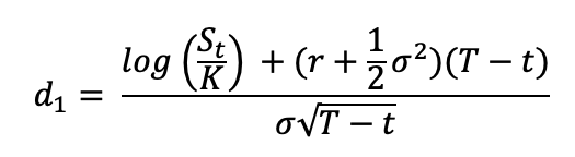
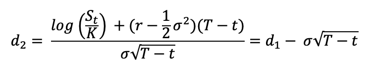
VIX index

In this article, Youssef LOURAOUI (ESSEC Business School, Global Bachelor of Business Administration, 2017-2021) presents the VIX index, which is a financial index that measures the uncertainty in the US equity market.
This article is structured as follows: we begin by defining the grounding notions of the VIX index. We then explain the behavior of this index and its statistical characteristics. We finish by presenting its practical usage in financial markets.
Definition
The CBOE Volatility Index, abbreviated “VIX”, is a measure of the expected S&P 500 index movement calculated by the Chicago Board Options Exchange (CBOE) from the current trading prices of options written on the S&P 500 index.
Known as Wall Street’s “fear index”, the VIX is closely monitored by a broad range of market players, and its level and pattern have become ingrained in market discussion.
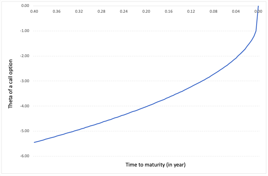
Figure 1 illustrates the evolution of the VIX index for the period from 2003 to 2021.
Figure 1 Historical levels of the VIX index from 2003-2021.
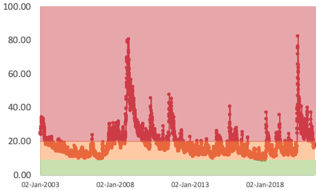
Source: computation by the author (Data source: Thomson Reuters).
VIX values greater than 20 are regarded to be high by market participants. If the VIX is between 12 and 20, it is considered normal; if it is less than 12, it is considered low. As it is the case with other indices, the VIX is computed using the price of a basket of tradable components (in this case, options expiring within the next month or so). The profit or loss that option buyers and sellers realize during the option’s life will depend, among other things, on how significantly the S&P 500’s actual volatility will differ from the implied volatility given by the VIX at the start of the period (S&P Global Research, 2017).
Behavior of the VIX index
Statistical distribution of the S&P500 index returns and VIX level
Figure 2 displays the statistical distribution of the price variations in the S&P500 index for different levels of the VIX index The higher the VIX index (by convention, greater than 20), the more severe the distribution tends to be, with negative skewness and high kurtosis indicating heightened volatility in the US market, therefore exacerbating both positive and negative swings. An opposite finding may be made for the VIX level at lower levels (often less than 12), when market swings are less evident due to less skewness and lower kurtosis (S&P Global Research, 2017).
Figure 2. The distribution of 30-day return in the S&P500 index for different VIX index levels.
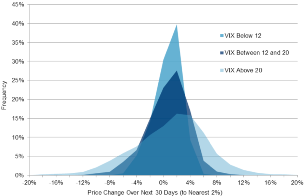
Source: S&P Global Research (2017).
If the VIX is low, market players may benefit by purchasing options; conversely, if the VIX is high, market participants may profit from selling options. The specific utility of anticipated VIX is that it gives us with a more accurate assessment of whether VIX is high, low, or normal at any point in time (S&P Global Research, 2017). Thus, VIX may be regarded of as a crowd-sourced estimate of the S&P 500’s expected volatility. As with interest rates and dividends, one cannot invest directly in them, even though one can guess on their future worth, one cannot invest directly in VIX, and the significance of a specific VIX level is commonly misinterpreted (S&P Global Research, 2017).
Recent volatility in the S&P500 index and VIX level
Figure 3 demonstrates that the VIX index is strongly correlated with recent market volatility. However, there is considerable variance; for example, a recent volatility level of about 20% has been associated with a VIX level of 34 (point B, when VIX was very “high”) and with a VIX level of 12 (point C, when VIX was relatively “low”). Volatility (realized or implied) has a strong propensity to return to its mean. This insight is not especially original, despite its illustrious past. There is an enormous body of data demonstrating that volatility tends to mean revert across markets, and the pioneers of this field were given the Nobel Prize in part for incorporating their results into volatility forecasts and simulations (S&P Global Research, 2017).
Figure 3. Relation between VIX and recent volatility.
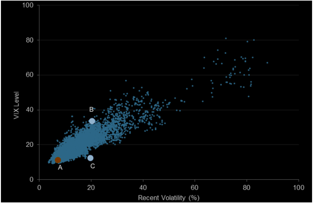
Source: S&P Global Research (2017).
Realized volatility in the S&P500 index and VIX level
Figure 4 represents the relationship between Realized volatility in the S&P500 index over a period and the VIX level at the begining of the period.
Figure 4. VIX versus next realized volatility.
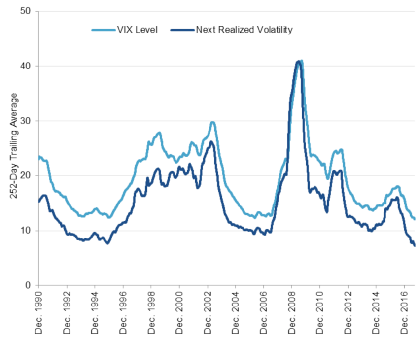
Source: S&P Global Research (2017).
Mean reversion
Figure 5 shows how VIX index converge to a certain llong-term level as time passes. This finding is not due to 15% being exceptional in any manner; this figure for M was calculated using historical volatility levels for the S&P 500 and their evolution. It is not implausible that M (else referred to as long-term average volatility in the US equities market) may change over time; changes in the S&P 500’s sector weightings, trade All of these factors have the ability to influence both the pace and the volume and the point at which mean reversion occurs.
Figure 5. Mean-reversion dynamic in recent volatility.
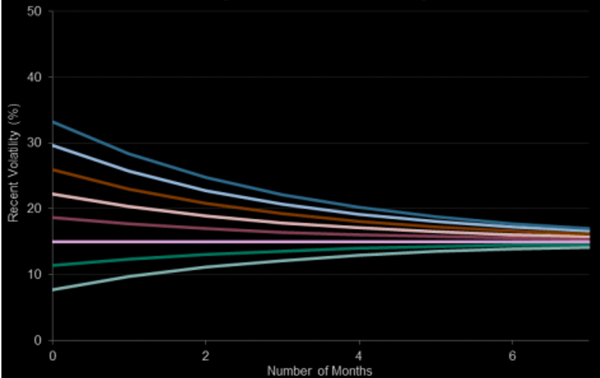
Source: S&P Global Research (2017).
Use of the VIX index in financial markets
There are two methods for determining an asset’s volatility. Either through a statistical calculation of an asset’s realized volatility, also known as historical volatility, which serves as a pointer to the asset’s volatility behavior. This is a limited method that is based on the premise that past volatility tends to replicate itself in the future, without including a forward-looking study of volatility. The second technique is to extract an asset’s volatility from option prices referred to as “implied volatility”.
Why should I be interested in this post?
When investors make investment decisions, they utilize the VIX to gauge the degree of risk, worry, or stress in the market. Additionally, traders can trade the VIX using a range of options and exchange-traded products, or price derivatives using VIX values.
Related posts on the SimTrade blog
▶ Akshit GUPTA Options
▶ Akshit GUPTA History of Option Markets
▶ Jayati WALIA Implied Volatility
▶ Youssef LOURAOUI Minimum Volatility Factor
Useful resources
Business analysis
CBOE , 2021. VIX
Nasdaq, 2021. Realized Volatility
Nasdaq, 2021. Vix Index Volatility
S&P Global Research, 2017. Reading VIX: Does VIX Predict Future Volatility?
S&P Global Research, 2017. A Practitioner’s Guide to Reading VIX
About the author
The article was written in September 2021 by Youssef LOURAOUI (ESSEC Business School, Global Bachelor of Business Administration, 2017-2021).