SimTrade blog -

Trading as Principal in Illiquid Markets: What No Finance Course Can Fully Prepare You For

July 24, 2026 by Isaac FAINSTEIN

In this article, Isaac FAINSTEIN, Director at Petrini Valores and Visiting Lecturer at IESEG School of Management (Lille), shares his professional experience as a trader in illiquid fixed income and emerging markets — and what practitioners know that most finance courses never cover.

About Petrini Valores

Petrini Valores is an Argentine broker-dealer specializing in fixed income, equities, derivatives, and financing. The firm operates as a market maker in illiquid corporate and provincial bonds, across multiple asset classes: peso-denominated, USD-denominated, inflation-linked, and dollar-linked instruments. It also participates as a member of underwriting syndicates in primary bond issuances.

As Director of the trading desk, I am responsible for pricing, execution, and risk management across these asset classes on a daily basis.

Logo of Petrini Valores.

Source: Petrini Valores.

Trading in practice: what the desk actually looks like

I have been trading fixed income and foreign exchange in Argentine markets for over fifteen years. Over that same period, I have taught applied finance courses at IESEG School of Management in Lille — courses built around the situations I encounter at the desk every week. What follows is an attempt to bridge those two worlds.

Agency, intermediation, and principal trading: three different jobs

Most finance programs teach students how to price securities. Fewer teach them what it actually feels like to put the firm’s capital at risk to make a market. The distinction between agency trading, intermediation, and principal trading is more consequential than most courses suggest.

In agency trading, you act on behalf of a client — executing their order in the market, taking no position yourself, earning a fee for the service. The client bears the market risk. You are their agent.

Intermediation — what practitioners often call riskless principal — is already a form of proprietary trading, technically speaking. You act as principal on both legs: you buy from one counterparty and simultaneously sell to another, earning the bid-ask spread. Because both legs close at the same time, your market exposure is minimal. You are not an agent of either side. You are a counterparty to both, just briefly, and without meaningful inventory risk.

Principal trading with inventory risk is something else entirely. The firm puts its own capital on the line with no guaranteed exit. You buy a bond from a client with no buyer lined up on the other side. You sell from your own inventory because a client needs to buy. You absorb the spread — and the full market risk that comes with holding the position until you can unwind it. The longer you hold, the more exposure you carry. This is the mode that no simulation fully replicates, and the one this article is about.

Pricing illiquid bonds: when there is no obvious answer

A large portion of my daily activity involves corporate and provincial bonds that do not trade on a liquid exchange. There is no visible order book. There is no Bloomberg mid-price that everyone agrees on. There is a fragmented OTC market where each dealer forms their own view of value.

When a client calls and asks for a bid or offer on one of these bonds, I have to produce a price — quickly, without full information. I know what I think the bond is worth. What I do not know is whether the client is a buyer or a seller.

This asymmetry is at the heart of market-making in illiquid securities. If I quote too tight a spread, I may find myself on the wrong side of a pre-arranged trade. A client may call five dealers simultaneously, collect our offers, and hit the best one — while already having a buyer on the other side paying more than my offer. In that case, I have sold bonds below what the market was willing to pay, and the client has effectively traded through me.

I use this scenario in class regularly. Students are always surprised. They assume that being a good trader means knowing what something is worth. It does — but it also means understanding the information game you are playing with the person on the other side of the phone.

Then there is the moment that every trader knows: you have priced the trade, the client has everything they need to decide, and then — nothing. They go to lunch. They are in a meeting. They are closing another trade. You are sitting there holding a price in a moving market, watching the bid shift while you wait for a response that may or may not come. No simulation I have seen fully replicates the specific discomfort of that moment.

Primary market underwriting: when commitment meets reality

Beyond secondary market activity, I participate as an underwriter in primary bond issuances for Argentine corporates, as part of the underwriting syndicate organized around each deal. This is a different kind of principal risk — one that is taken on before the bond even exists.

When a company decides to issue a bond, I commit to underwriting a portion of the deal. This is a real financial commitment: if investor demand is insufficient to cover the full issuance, I absorb the remainder onto my own book. In Argentina, primary markets typically use a Dutch auction format — investors submit bids specifying the coupon rate they are willing to accept and the quantity they want. The issuer then sets a clearing rate that satisfies the target issuance amount.

On auction day, I am simultaneously placing bonds with my own client base, managing my underwriting exposure, and monitoring where the clearing rate is likely to land. If I have covered my commitment with investor demand, I am in good shape. If not, the unsold portion of my underwriting commitment ends up on my balance sheet at the clearing rate — and I work that position off over the following days or weeks, offering it into a market that may or may not be ready to absorb it.

This is textbook principal risk. It is also something that very few students have any mental model for before entering the industry.

FX mismatches and capital controls: the Argentine laboratory

Argentina has operated with capital controls for years. At their peak, the gap between the official exchange rate and the blue-chip swap rate — a market-implied rate derived from the implicit FX embedded in cross-market bond transactions — reached several hundred percent. Today the gap has narrowed significantly, but the structure remains.

This creates situations that no standard finance course addresses. A bond denominated in dollars can be bought and sold in different currencies. If I buy a USD bond paying dollars and sell it against pesos, I receive pesos for an asset I paid for in dollars. I now have a currency mismatch on my book: I am effectively long pesos, short dollars. I can hedge that exposure immediately by buying back the dollars in the FX market, or — if I have a view that the implied exchange rate will move in my favor — I can hold the position and let it run.

The decision is not mechanical. It depends on my reading of the regulatory environment, the direction of the blue-chip swap rate, and how much currency risk I am willing to carry on the book at that moment. This is daily life on the desk. And it is very difficult to teach without the context that produces it.

When models break: the lesson of negative oil prices

In April 2020, front-month WTI crude oil futures briefly traded at negative prices. Physical storage constraints had overwhelmed the market’s mechanics, and sellers were willing to pay counterparties to take delivery of crude oil they had nowhere to store.

I watched it happen from the desk in real time. What struck me was not the price itself — it was the reaction across the industry. Many traders assumed it was a glitch. Some platforms were simply not built to display or process negative prices, and brokers whose systems could not show the quotes found themselves liable to clients who could not see — let alone act on — what was happening in the market. Several firms had to absorb losses because their technology had never contemplated the possibility.

I use this episode as an opening in class — not to explain futures mechanics, which students can read in any textbook — but to ask a different question: what do you do when the model produces an answer that the real world seems to reject? What is your decision framework when your screen shows something that looks impossible? The answer is that you need to understand the why behind the price before you can act on it. That understanding is not something you can look up in real time. Either you have built it, or you have not.

The most important rule on a trading desk

Every trader makes mistakes. A wrong-way position, a misread signal, a fat-finger entry. What separates good trading culture from bad is not the absence of errors — it is what happens in the first thirty seconds after one occurs.

The worst thing a trader can do is wait. Hiding a mistake, even briefly, turns a manageable problem into a serious one. A position that could have been closed at a small loss will compound. The bid-ask spread you avoided paying once will have widened by the time you are forced to act.

The most important rule on any trading desk is this: when you make a mistake, communicate it immediately. No fear of consequences should outweigh the cost of silence. A well-run desk creates an environment where immediate transparency is rewarded — because the alternative is invariably more expensive. This is not a financial concept. It is a cultural one. And it may be the most practically useful thing I can tell any student before they sit down at a real trading desk for the first time.

Argentina: the best trading school you never attended

With a World Cup recently concluded — and Argentina’s performance still fresh in everyone’s memory — there is a useful analogy worth making. Argentina’s best players did not all come through polished academies with perfect pitches and controlled conditions. Many learned on uneven surfaces, in chaotic environments, where improvisation and resilience were not optional. Those conditions, more often than not, produced technically complete and mentally durable players.

The same logic applies to trading in an environment like Argentina. Multiple asset classes, multiple yield curves, structural illiquidity, capital controls, and macroeconomic volatility — all simultaneously, all the time. Traders who come through this market and move to larger ones — Brazil, Mexico, or developed markets — typically find the transition smoother than expected. They have already navigated conditions that most traders in more liquid markets never face. When you learn to trade in the mud, the rest feels like solid ground.

Financial concepts related to this article

I present below four financial concepts central to my daily work as a trader in illiquid and emerging markets.

Principal trading and inventory risk

In principal trading, the broker-dealer buys or sells securities using its own capital, taking market risk onto its own balance sheet. This contrasts with agency trading, where the firm executes on behalf of a client and earns a fee, or with intermediation (riskless principal), where the firm matches both sides simultaneously and earns the bid-ask spread without holding inventory risk. The critical difference is time: in principal trading, the firm holds a position that may not be unwound immediately, and the longer it is held, the greater the market exposure.

Underwriting syndicate and book runner

In a primary bond issuance, several broker-dealers form an underwriting syndicate, each committing to place a portion of the deal with investors. The book runner is the lead of this syndicate — it manages the investor order book, coordinates pricing with the issuer, and oversees the allocation process. Other syndicate members, such as Petrini Valores in many Argentine corporate issuances, commit to their own underwriting tranche and are responsible for placing it with their client base. If a syndicate member cannot fully place its portion, the unsold bonds remain on its balance sheet at the clearing rate.

Dutch auction in primary bond markets

A Dutch auction is a price-discovery mechanism in which investors submit bids specifying both quantity and the coupon rate they are willing to accept. The issuer sets a single clearing rate that satisfies the target issuance amount. All successful bidders receive bonds at the clearing rate, regardless of their individual bids. This format is widely used in Argentine primary markets for corporate bond issuances.

Blue-chip swap rate and capital controls

In markets with capital controls, such as Argentina, the blue-chip swap rate (also known as the contado con liquidación or CCL rate) is an implied exchange rate embedded in cross-market bond transactions. It reflects the market’s assessment of currency value in the absence of free convertibility and can diverge significantly from the official rate. Managing positions across currencies in this environment requires an understanding of the regulatory framework and a constant read on the gap between official and market-implied rates.

Why should I be interested in this post?

If you are a finance student planning to work in sales and trading, fixed income, or any market-facing role, the situations described here are among the ones you will encounter earliest — and none of them are fully captured in a simulation or a pricing model.

The gap between finance education and market reality is not about knowledge. Most graduates know their bond math. The gap is about judgment: knowing how to act when information is incomplete, the counterparty is not responding, and the market is moving. Understanding how principal risk, illiquidity, and currency mismatches interact in real time is the difference between arriving prepared and arriving surprised.

Useful resources

Academic research

Gkillas K. and Longin, F. (2018) Financial market activity under capital controls: lessons from extreme events, Economics Letters, 171, 10-13.

Martellini, L., Priaulet, P., Priaulet, S. (2003) Fixed-Income Securities: Valuation, Risk Management and Portfolio Strategies, John Wiley & Sons.

Hull, J. C. (2021) Options, Futures, and Other Derivatives, 11th edition, Pearson.

Business resources

Petrini Valores — Argentine broker-dealer specializing in fixed income, equities, derivatives, and financing.

FINRA Tools and Calculators — public source for US bond transaction data and pricing context.

About the author

This article was written in July 2026 by Isaac FAINSTEIN, Director at Petrini Valores and Visiting Lecturer at IESEG School of Management (Lille), where he has taught applied finance and trading courses for over 10 years.

▶ Discover all articles by Isaac FAINSTEIN.

Delta Hedging Explained: How Traders Stay Market Neutral

July 23, 2026 by Abel ARAYA

In this article, Abel ARAYA (ESSEC Business School, Master in Finance, 2025) takes a detailed and practical look at delta hedging, a core concept in options trading. Far from being just a mathematical tool, delta hedging is a real-world technique that allows traders to manage market risk dynamically and stay focused on what they actually want to trade: volatility and relative value.

Understanding the challenge of options trading

When a trader buys or sells options, they are taking a view not only on the direction of the market but also on how much the market might move. The value of an option changes constantly, influenced by multiple factors such as the price of the underlying asset, time decay, volatility, and interest rates. Without active management, these continuous changes can make an options book risky and unpredictable.

Delta hedging addresses this by adjusting the position in the underlying asset to neutralize the impact of small price movements. The trader aims for a portfolio that reacts as little as possible to minor changes in the underlying price so that risk is concentrated on the variables they intend to trade, such as volatility.

What exactly is delta?

Delta is one of the key Greeks that measure how the price of an option responds to changes in market variables. It tracks the sensitivity of the option value to the underlying price.

Δ = ∂V / ∂S

Here, V is the option value and S is the price of the underlying asset. For example, if a call option has a delta of 0.60, a rise of 1 euro in the underlying increases the option value by about 0.60 euro. A delta close to 1 behaves like the underlying, while a delta near 0 barely reacts to price moves.

The principle of delta neutrality

Suppose a trader has sold call options on a stock. If the stock rises, the calls gain value and the short position loses money. To offset this exposure, the trader buys shares of the underlying. The goal is to hold a number of shares that compensates the option’s delta so that small moves in the stock price do not change the portfolio value.

Δ_portfolio = Δ_option + Δ_hedge = 0

The trader dynamically buys or sells the underlying to keep the combined delta close to zero.

The dynamic nature of delta

Delta changes as markets evolve, time passes, or volatility shifts. The speed of this change is captured by gamma, which measures the curvature of the option value with respect to the underlying price.

Γ = ∂²V / ∂S²

A high gamma means delta changes quickly, which forces more frequent rebalancing. Large options books can require several adjustments per day during volatile periods. In episodes of market stress, hedging flows can increase significantly as deltas move rapidly.

Hedging a single option versus a book of options

So far we have described delta hedging for a single option, but a trader on a derivatives desk rarely manages one position in isolation. In practice, the desk holds a book of hundreds or thousands of options across many underlyings, strikes and maturities. Hedging each one separately would be inefficient and very costly in transaction fees.

Instead, the trader looks at the net risk of the entire book. All the individual deltas are aggregated into a single net delta for the portfolio, and only that net exposure is hedged in the underlying. Long and short positions offset each other, so the desk usually needs far fewer hedging trades than the number of options it holds. The same logic applies to the other Greeks: the book is managed at the level of its net delta, gamma and vega rather than option by option. This portfolio approach is what makes running a large options book possible, and it is one of the core skills of a derivatives trader.

Re-hedging and trading costs

Each rebalancing operation generates transaction costs, including bid-ask spreads and slippage. Skilled traders balance precision and efficiency, deciding when to rebalance and when to tolerate a small residual exposure. Frequent re-hedging reduces risk but can erode profits through costs. The optimal approach depends on liquidity, volatility, and position size.

Why delta hedging matters

Delta hedging allows traders to isolate the risks they want to trade. By neutralizing directional exposure, they can focus on volatility, time decay or interest rate sensitivity. For instance, a volatility trader may be long options but delta-hedged, seeking to profit if realized volatility exceeds implied volatility rather than from market direction.

Securing the bank’s margin

For a bank acting as a market-maker, delta hedging is not only a risk-management tool: it is also what allows the desk to secure its margin. When the bank sells an option to a client, it charges a price that is slightly above the option’s theoretical, or fair, value given by its pricing models. That difference between the price paid by the client and the theoretical value is the bank’s margin.

By delta hedging the position dynamically, the bank replicates the payoff of the option at a cost close to its theoretical value while neutralizing the impact of market direction. If the hedging is done well, the bank is no longer betting on whether the underlying goes up or down: it has locked in that initial margin regardless of how the market moves. In other words, delta hedging turns a directional exposure into a controlled activity whose objective is to capture and protect the spread between the price sold to the client and the theoretical value of the option.

A practical example

Consider a trader who sells 5 million euros of call options on the EuroStoxx 50 with an average delta of 0.4. To stay neutral, the trader buys 2 million euros of EuroStoxx 50 futures, which offsets the option delta. If the index rises and delta increases, the trader buys more futures. If it falls, they reduce the hedge. The objective is to end the day with minimal unhedged exposure despite continuous fluctuations.

Although the mechanics look simple, judgment matters. On quiet days, fewer adjustments are needed. In unsettled markets, hedging becomes more frequent. Delta hedging therefore blends quantitative discipline with trader intuition.

Common misconceptions

Delta hedging does not eliminate all risk. It removes first-order sensitivity to small price moves. Sudden jumps in price or volatility introduce residual risks captured by higher-order Greeks such as gamma and vega. Effective options risk management considers these dimensions together.

Conclusion

Delta hedging is a practical cornerstone of modern options trading. By continuously adjusting exposure, traders can focus on pricing, volatility and liquidity rather than guessing direction. Understanding delta hedging provides a clearer view of market neutrality in practice.

Why should I be interested in this post?

If you are a student in finance interested in derivatives, trading, or risk management, delta hedging is one of the most fundamental concepts you will encounter in practice. It bridges the gap between option pricing theory and what traders actually do every day on the floor. Understanding delta hedging will give you a concrete language for discussing risk with traders and structurers in interviews, and it directly underpins roles in equity derivatives, rates options, and exotic products desks.

More broadly, the logic of delta hedging, isolating a risk you want to trade from one you do not, applies far beyond options. It is central to how banks and hedge funds manage their books across all asset classes. Whether you are targeting a front-office internship, a quant role, or a risk management position, mastering this concept will give you a genuine edge.

Useful resources

Hull J.C. (2022) Options, Futures, and Other Derivatives, Pearson, 11th Edition.

Black F. and Scholes M. (1973) The Pricing of Options and Corporate Liabilities”, Journal of Political Economy, 81(3), 637-654.

Merton R.C. (1973) Theory of Rational Option Pricing Bell Journal of Economics, 4, 141–183.

Bank for International Settlements — OTC Derivatives Statistics

About the author

The article was written in July 2026 by Abel ARAYA (ESSEC Business School, Master in Finance, 2025).

▶ Discover all articles by Abel ARAYA

Inside the Markets COO Office at HSBC: Understanding How Trading Floors Are Managed

July 23, 2026 by Abel ARAYA

In this article, Abel ARAYA (ESSEC Business School, Master in Finance, 2025) offers an inside look at the Markets COO Office at HSBC Continental Europe. Through his one-year apprenticeship, he shares how this central function coordinates trading activities, manages budgets and risks, and ensures that the Markets division operates with efficiency and strategic discipline.

About the company

HSBC was founded in 1865 as the Hongkong and Shanghai Banking Corporation to finance trade between Europe and Asia, and has since grown into one of the world’s leading financial institutions. Headquartered in London and listed in London, Hong Kong, New York, Paris and Bermuda, it held around 3.2 trillion US dollars in assets at the end of 2025, employed roughly 211,000 people across some 56 countries and territories, and served more than 40 million customers.

On the wholesale side, its corporate and institutional clients are covered by the Corporate and Institutional Banking (CIB) division, which generated around 27.6 billion US dollars in revenue in 2025. Within CIB, the Markets and Securities Services teams provide liquidity, financing and risk-management solutions across fixed income, credit, FX, equities and securities services to large corporates, financial institutions, asset managers, hedge funds and governments. In this business HSBC competes with the other major global markets houses, such as JPMorgan, Citi, Bank of America and Goldman Sachs in the United States, and Deutsche Bank, Barclays, BNP Paribas and Société Générale in Europe, differentiating itself through its international network and its historical strength in Asia.

I worked at HSBC Continental Europe, the group’s Paris-headquartered subsidiary covering continental Europe. Since the sale of its French retail banking business on 1 January 2024, it has refocused on corporate and institutional clients, with a consolidated balance sheet of 251 billion euros in total assets at the end of 2025.

Logo of HSBC.

Source: the company.

During my apprenticeship, the Markets division was in the process of being integrated into the broader Corporate and Institutional Banking (CIB) structure. This reorganization involved significant changes to how the division was managed, reported, and resourced, which made my experience at the COO Office particularly rich in terms of exposure to strategic and operational transformation.

My internship

My missions

As a Business Manager Assistant within the Markets COO team, my work covered a wide range of financial and operational responsibilities. I contributed to the production of internal reports and presentations for senior management, summarizing the performance, expenses, and headcount of the Markets division. These documents were used in management meetings, financial steering committees, and due diligence reviews conducted during the restructuring process.

I was closely involved in cost forecasting and budget follow-up, helping the team anticipate upcoming expenses and identify deviations from plan. One of my key projects was the annual broker review, which required consolidating trading flow data across all asset classes to assess the efficiency, transparency, and compliance of relationships with external counterparties. This involved close coordination with traders, operations, and compliance teams across Paris, Germany, and India.

I also supported the preparation of headcount reports and organizational charts used by senior management to steer the restructuring of the division. These deliverables required precision and a thorough understanding of how each desk contributed to the overall structure of the Markets business.

Required skills and knowledge

This role required a combination of analytical and interpersonal skills. On the technical side, strong proficiency in Excel was essential for building budget models, consolidating large datasets, and producing financial summaries. Familiarity with the structure of a markets division, including the roles of front office, operations, compliance, and finance, was also important to contextualize the data I was working with.

Soft skills mattered just as much. Coordinating with stakeholders across multiple countries and hierarchies required clear written and oral communication, the ability to manage competing priorities, and a high level of attention to detail. The pace of the environment also demanded adaptability: priorities shifted quickly, and producing reliable output under time pressure was a daily reality.

What I learned

This experience gave me a deep understanding of how financial institutions manage their operations behind the scenes. I learned how budgets are built, how costs are tracked and challenged, and how strategic decisions made at senior level translate into concrete actions on the trading floor. I also developed a much clearer picture of how risk is monitored and how compliance frameworks shape the day-to-day behaviour of a markets division.

Working across teams in Paris, Frankfurt, and India gave me direct exposure to how global coordination works in practice. I learned the importance of data quality and rigour: a single inconsistency in a report could lead to misunderstandings or delayed decisions at the highest level. This reinforced my attention to detail and my commitment to producing work that is both accurate and clearly communicated.

Financial concepts related to my internship

I present below three financial concepts related to my internship: cost and budget management, change management, and due diligence.

Cost and Budget Management

Cost and budget management refers to the process by which an organization plans, monitors, and controls its financial resources to ensure that spending remains aligned with strategic objectives. In a markets division, this involves tracking a wide range of costs: staff compensation, technology infrastructure, external service providers, and regulatory compliance expenses. The budget is typically set at the beginning of the year based on business forecasts and strategic priorities, and then monitored on a monthly basis against actual expenditure.

In my role at the Markets COO team, cost and budget management was one of my primary responsibilities. I contributed to the monthly budget follow-up by consolidating cost data from different desks and entities, identifying variances between forecasts and actual figures, and preparing summary reports for senior management. When a desk was running significantly above or below budget, the COO team would investigate the drivers and, if necessary, escalate to management for a decision. I learned that in a large institution like HSBC, even small deviations in cost forecasts can have a significant impact on the division’s overall financial performance, particularly during a period of restructuring where cost targets were closely scrutinized.

Change Management

Change management is the structured approach through which an organization transitions from its current state to a desired future state while minimizing disruption to operations and people. In the context of financial institutions, it often involves reorganizations, mergers of business lines, technology migrations, or regulatory-driven transformations. Effective change management requires clear communication, stakeholder alignment, and careful sequencing of decisions to ensure continuity of service during the transition.

During my apprenticeship, HSBC’s Markets division was undergoing a major strategic restructuring: the Markets and Securities Services unit was being integrated into the broader Corporate and Institutional Banking (CIB) structure. This was not a minor adjustment, but a fundamental reorganization of how the division was governed, resourced, and reported. I observed the effects of this transformation directly through my work: headcount reports were being revised regularly, cost allocation frameworks were changing, and the responsibilities of the COO team were evolving to reflect the new organizational model. I worked closely with the COO based in Germany, who was managing part of this transition, and I saw first-hand how much coordination and precision are required to keep a large division functioning smoothly while simultaneously reshaping it. Change management, in that context, was not an abstract concept: it was a daily operational reality.

Due Diligence

Due diligence refers to the comprehensive process of investigating and verifying information before making a significant business decision. In investment banking and financial services, it is most associated with mergers and acquisitions, where a buyer conducts a thorough review of the target company’s finances, legal situation, and operations. However, the concept applies equally to other contexts, including the assessment of external service providers, the validation of financial data before it is presented to management, and the review of counterparty relationships.

In my role, due diligence took the form of the annual broker review process. This involved systematically reviewing the trading flows directed to each external broker, verifying the accuracy of the data, and assessing whether the allocation of business to each counterparty was justified by objective performance criteria. The process required gathering data from multiple sources, reconciling inconsistencies, and presenting findings to senior management with clear supporting evidence. I also contributed to due diligence exercises conducted during the restructuring process, where the COO team was asked to validate headcount and cost data before it was presented to the executive committee. These experiences taught me that rigorous due diligence is not just about finding problems: it is about building the trust and confidence that allow organizations to make well-informed decisions.

Why should I be interested in this post?

If you are a student in business and finance considering a career in financial markets, this post offers a perspective that is rarely covered in mainstream discussions about finance careers: the operational and strategic backbone of a trading floor. Most students aspire to front-office roles in trading or sales, and rightly so. But understanding how a markets division is actually run, how its costs are managed, how its risks are monitored, and how major transformations are navigated, is an invaluable foundation for any finance career.

A role in a Markets COO or Business Management team is particularly well-suited for students who want to develop a transversal understanding of markets while building strong analytical and organizational skills. It is also increasingly recognized as a credible path toward front-office positions: many senior traders and sales managers have spent time in COO or control functions early in their careers, and this experience gives them a level of business awareness that pure front-office profiles often lack. Whether you are targeting trading, sales, risk, or corporate finance, the skills and perspective gained in this type of role will give you a genuine advantage.

Useful resources

HSBC — Corporate and Institutional Banking

ESMA — MiFID II and MiFIR

Basel Committee on Banking Supervision — Sound Practices for Operational Risk Management

About the author

The article was written in July 2026 by Abel ARAYA (ESSEC Business School, Master in Finance, 2025).

▶ Discover all articles by Abel ARAYA

What I Learned on a Trading Floor at HSBC: Understanding Markets from the Inside

July 23, 2026 by Abel ARAYA

In this article, Abel ARAYA (ESSEC Business School, Master in Finance, 2025) shares his experience on HSBC’s trading floor in Paris. He explains how this opportunity helped him understand how a global markets division operates, how teams interact, and what makes the environment of a trading floor so unique.

From private banking to markets

Before joining HSBC, I was working in private banking at Milleis Banque Privée. It was a good introduction to finance, but I wanted to understand how the markets worked behind the scenes. Joining HSBC Continental Europe as a Business Manager Assistant within the Markets COO (Chief Operating Officer) team gave me the chance to discover that world for the first time. The COO function within a markets division is responsible for the operational and financial oversight of the trading floor: it sits at the intersection of strategy, finance, and day-to-day management, supporting the front office without being directly involved in trading itself.

About the company

HSBC was founded in 1865 as the Hongkong and Shanghai Banking Corporation, created to finance trade between Europe and Asia. More than a century and a half later, it has become one of the largest banking and financial services groups in the world. Headquartered in London and listed in London, Hong Kong, New York, Paris and Bermuda, the group held around 3.2 trillion US dollars in assets at the end of 2025, employed roughly 211,000 people across some 56 countries and territories, and served more than 40 million customers.

On the wholesale side, where I worked, HSBC brings together its corporate and institutional clients under the Corporate and Institutional Banking (CIB) division, which generated around 27.6 billion US dollars in revenue in 2025. CIB was created on 1 January 2025 by combining the former Global Banking and Markets business with commercial banking activities outside the UK and Hong Kong, with the ambition of ranking among the top three global wholesale banks. Within CIB, the Markets and Securities Services teams provide liquidity, financing and risk-management solutions across fixed income, credit, foreign exchange, equities and securities services.

Its clients are large corporates, financial institutions, asset managers, hedge funds and governments that rely on the bank to trade, hedge and finance their activities across the world. In this space HSBC competes with the other large global markets houses, such as JPMorgan, Citi, Bank of America and Goldman Sachs in the United States, and Deutsche Bank, Barclays, BNP Paribas and Société Générale in Europe. Its main differentiator remains its international network and its historical strength across Asia and emerging markets.

My apprenticeship took place at HSBC Continental Europe, the group’s Paris-headquartered subsidiary covering continental Europe. Since the sale of its French retail banking business on 1 January 2024, HSBC Continental Europe has refocused on corporate and institutional clients, with a consolidated balance sheet of 251 billion euros in total assets at the end of 2025.

During my apprenticeship, this reorganization was still under way, which made it a particularly interesting time to observe how such a large organization adapts its structure while continuing to run its business day to day.

Logo of HSBC.

Source: the company.

My apprenticeship

Within the Markets COO team, my work focused on the financial and organizational aspects of the trading floor. I contributed to budget monitoring, forecasts of upcoming expenses, and internal reports related to costs and resources. I was involved in the broker review process and in the preparation of financial summaries presented to management.

This position gave me a transversal view of the Markets division and helped me understand how each team contributes to the overall structure. I interacted with many different stakeholders: the COO in Germany, who was managing a restructuring process, teams in India working on operational data, and senior managers in Paris overseeing the desks. These collaborations taught me how coordination and communication are essential to keep such a large platform running efficiently.

Life on the trading floor

Working so close to the trading floor was one of the most rewarding parts of my experience. Even though my role was on the management side, I was constantly in contact with the desks. I often visited traders, salespeople, and structurers to better understand their activities and the financial implications of their operations. One moment that stayed with me was a conversation with a rates trader during a period of elevated volatility in the European bond market. He explained how the sudden widening of spreads between Italian BTPs and German Bunds was forcing him to adjust his hedging positions in real time, something I had only ever read about in textbooks. These interactions helped me connect the numbers I was analysing to the real market dynamics they represented.

The atmosphere on the floor was intense and collaborative at the same time. Information flowed constantly between desks, from rates to credit to repo, and decisions were made quickly. Observing this rhythm every day helped me understand how interconnected market teams are, and how much relies on clear communication and mutual trust.

What I learned

This experience gave me a real understanding of how a trading floor operates, both economically and humanly. I learned how a large institution like HSBC manages its costs, allocates resources, and balances strategic priorities with budget realities. I also saw how economic pressures, regulatory changes, and internal dynamics influence decisions at every level of the organization.

Spending time close to the Fixed Income desks gave me a concrete sense of how sales, traders, and support teams work together. I realized that beyond products and numbers, markets are built on relationships, coordination, and constant adaptation.

Most importantly, this experience taught me the value of curiosity and initiative. By going to speak directly with teams, asking questions, and trying to understand their world, I gained insights that no spreadsheet could have given me. It made me appreciate both the complexity and the humanity of financial markets.

This one-year apprenticeship was a very strong first step into the world of markets. It helped me confirm that the natural next step for me would be a front-office internship as a Sales in Fixed Income, where I could build on what I learned and continue to grow within a trading environment.

Financial concepts related to my professional experience at HSBC

I present below three financial concepts related to my internship: market liquidity, collusion risk, and profit and loss (P&L).

Market Liquidity

Market liquidity refers to the ease with which a financial instrument can be bought or sold in the market without significantly moving its price. A liquid market has many buyers and sellers, tight bid-ask spreads, and the ability to execute large transactions quickly. An illiquid market, by contrast, forces participants to accept worse prices or wait, which can turn a theoretically profitable position into a loss once execution costs are taken into account.

In fixed income markets, liquidity is not uniform: it varies by product, by maturity, and by the time of day. Sovereign bonds such as French OATs or German Bunds are among the most liquid instruments in the world, with spreads of just a few basis points. Corporate bonds, by contrast, trade far less frequently and can see spreads widen dramatically in periods of stress. Structured products and exotic rates instruments can be even harder to unwind quickly.

One of the things I discovered at HSBC is the central role brokers play in providing liquidity. Not all brokers are equal: some are specialists on particular products or market segments. For example, inter-dealer brokers such as TP ICAP or Tradition are well known for their activity in rates and repo markets, where they connect banks anonymously to facilitate large transactions. During the annual broker review process that I participated in, traders would assess which brokers had provided the best liquidity, the most reliable pricing, and the fastest execution across different products. This review directly influenced how trading flows were allocated across brokers the following year. It made me understand that liquidity is not just a market property: it is also a relationship, built and maintained between institutions over time.

Collusion Risk

In financial markets, collusion risk between traders and brokers refers to a specific form of conflict of interest: a trader systematically routing a disproportionate volume of transactions to a particular broker, not because that broker offers the best execution, but because of a personal relationship, reciprocal favours, or informal arrangements. This behaviour is harmful to clients, who are entitled under regulation to receive the best available price and execution, a principle known as best execution, enshrined in the MiFID II directive in Europe.

The risk is subtle and not always easy to detect. A trader may genuinely believe that their preferred broker is the best, when in reality they are simply more comfortable with them. Over time, this can result in a concentration of flows toward one or two brokers that is not justified by objective performance criteria such as pricing quality, speed of execution, or market access. In the worst cases, the relationship can involve gifts, entertainment, or the sharing of confidential information, all of which are strictly regulated.

This is exactly what the annual broker review process at HSBC was designed to monitor and prevent. As part of my role in the Markets COO team, I contributed to this review, which involved analysing the distribution of trading flows across brokers and comparing it against objective performance metrics. If a trader was sending a significantly higher share of their volume to one broker without a clear justification, that anomaly would be flagged and discussed. The process ensured that broker relationships remained grounded in performance rather than personal preference, protecting both the bank and its clients. Working on this review gave me a direct understanding of how compliance and governance function in practice on a trading floor, and why they matter.

Profit and Loss (P&L)

Profit and Loss (P&L) is the daily measure of how much money a trading desk has made or lost. It captures the combined effect of market movements, trading activity, and fees. In my role within the Markets COO team, the P&L was one of the most important indicators I worked with. Each morning, the desks produced a flash P&L report, and my team consolidated these figures to produce management summaries that were reviewed by senior leadership. I also contributed to the analysis of P&L trends over time, identifying which desks were performing above or below forecast and understanding the drivers behind deviations. I learned that P&L is not just a financial result: it is a real-time signal of how well a desk is managing its positions, its risks, and its client relationships. Monitoring P&L every day gave me a concrete and dynamic view of how financial markets translate into business performance.

Why should I be interested in this post?

If you are a student in business or finance thinking about a career in financial markets, this post can help you understand what to expect from a first experience on a trading floor. Many students have a strong theoretical background in finance but are uncertain about how these concepts translate into day-to-day work. Through my experience at HSBC, I discovered that even a non-front-office role offers an exceptional vantage point: by working within the Markets COO team, I was exposed to P&L reporting, liquidity management, broker reviews, and budget processes that are central to how a bank manages its markets activities.

This post is also relevant if you are considering roles in Markets COO, Business Management, or Finance Control within a bank. These positions are often overlooked by students who focus exclusively on trading or sales, yet they offer direct exposure to the full scope of a markets division and are increasingly valued as a stepping stone toward front-office responsibilities. Whatever your target role, understanding how a trading floor operates, its rhythms, its pressures, and its culture, will give you a real advantage in interviews and on the job.

Useful resources

HSBC — Corporate and Institutional Banking (including Markets and Securities Services)

ESMA — European Securities and Markets Authority

BIS — OTC Derivatives Statistics

About the author

The article was written in July 2026 by Abel ARAYA (ESSEC Business School, Master in Finance, 2025).

▶ Discover all articles by Abel ARAYA

When custom software becomes a management decision

July 22, 2026July 22, 2026 by Axel RUDLOFF

In this article, Axel RUDLOFF (founder and President of Koragence, and a student at ESSEC Business School, Grande Ecole Program – Master in Management (MiM), 2025–2029) shares observations drawn from building and managing software engineering projects involving system integration, artificial intelligence (AI), DevOps and custom business applications. The article explains why a software project is not only a technical investment: it is also a managerial decision about productivity, risk, operating processes and capital allocation.

Introduction

Companies rarely decide to develop custom software when existing systems no longer support the way the business actually operates. An enterprise resource planning system (ERP), such as SAP, may need to exchange data with a customer relationship management system (CRM), supplier application programming interfaces (APIs), document-management tools or applications developed internally. Difficulties arise when these systems must share data reliably, enforce specific business rules and support critical processes without repeated manual entry.

At Koragence, the projects I supervise often involve synchronising ERPs, integrating partner APIs, automating document processing with AI, rebuilding business workflows, or implementing DevOps architectures. DevOps refers to the practices and tools used to automate, secure and monitor the development and operation of software. Depending on the business criticality of a project, the architecture may target 99.95% availability, or up to 99.99% when the infrastructure supports multi-region redundancy, load balancing and advanced incident-recovery mechanisms.

About Koragence

Koragence is a French digital-services company specialising in custom software, web engineering, and process automation. The company designs business applications, software-as-a-service (SaaS) platforms, internal tools, customer portals and technical integrations for companies, startups, associations and public organisations.

Koragence has delivered more than 20 projects for clients located in more than six countries and works with a network of more than 50 active collaborators and partner companies. This model makes it possible to assemble a team according to the specific needs of each assignment, including software development, user experience and user interface design (UX/UI), cloud infrastructure, cybersecurity, accessibility and data engineering.

Logo of Koragence.

Source: the company.

My experience as founder and President

As founder and President, I am responsible for turning a business problem into a project that can be delivered economically and technically. This includes business development, qualification of client needs, project scoping, pricing, team selection, contractual discussions, delivery governance and long-term client relationships.

I also remain directly involved in product and technical decisions. On a typical assignment, I help identify the critical workflow, define the minimum useful scope, choose which components should be standard and which should be custom, coordinate the specialists involved, monitor delivery and manage relationships with clients.

My main responsibilities

My work can be divided into five areas: identifying operational problems with measurable business consequences; translating those problems into functional and technical features; building the right project team; controlling scope, budget, quality and delivery risk; and ensuring that the software creates value after deployment rather than becoming an additional tool that employees do not use.

Required skills and knowledge

This role requires both technical and managerial skills. Technical knowledge is necessary to assess architecture, security, integrations, databases and infrastructure. Business knowledge is equally important because the best technical solution is not always the best investment. A founder must also understand margins, cash flow, pricing, negotiation, contractual risk and the opportunity cost of allocating a team to one project rather than another.

The most important soft skills are active listening, synthesis, communication and decision-making under uncertainty. Clients rarely describe their problem in technical terms. It is therefore necessary to distinguish symptoms from root causes, challenge assumptions with diplomacy, and explain trade-offs to both technical and non-technical stakeholders.

What I have learned

The main lesson is that the quality of the initial diagnosis, the clarity of responsibilities and the realism of the scope have a major impact on project cost and delivery.

The invisible cost of a fragmented information system

One of the most frequent problems is the repeated entry of the same information into several systems. In one project for an industrial group with several hundred employees, a team spent more than 1,600 hours per year re-entering information from supplier catalogues into an internal database. Beyond the labour cost, this process created entry errors, inconsistencies between reference systems and disputes caused by contradictory information.

The software project removed this break in the information flow. Supplier data were collected automatically through standardized AI document extraction, checked for consistency and integrated into the internal SAP system. The economic value came from reducing labour and disputes with suppliers.

Integration has become a central management issue

Suppliers increasingly expose APIs, ERPs provide connectors, CRMs publish webhooks and most business software can exchange data automatically. This creates opportunities, but every external connection also becomes a dependency. A partner API may change version, become unavailable or modify its behaviour. Reliable software therefore requires monitoring, logging, error recovery, security controls and ongoing maintenance.

In another project, Koragence developed a platform capable of supervising more than 15 industrial machines through supplier APIs while centralising more than 1,100 alerts and distributing notifications across several channels. The architecture was designed to scale to 100 machines without replacing the underlying technical model.

This type of project illustrates why integration is a strategic issue. The system must not only work on launch day; it must continue to work when the number of users, machines, documents or external dependencies increases. Maintenance is therefore part of the investment decision from the beginning.

Artificial intelligence changes the economics of software and automation

In the past, automating supplier catalogues, technical data sheets, invoices and other documents required highly standardised formats and rules written separately for each source. In practice, these standards were often incomplete or inconsistently applied. AI models can now interpret a much wider variety of documents, extract useful information and feed databases or business software. This makes some automations faster and less expensive to implement.

However, AI does not remove the need for architecture, control and human judgment. A 2026 study of more than 100,000 software developers found that autonomous coding agents produced very large gains in coding activity, but smaller gains at the level of completed projects and actual releases. The authors interpret this difference as evidence that human and organisational bottlenecks still limit final output. In other words, writing code faster does not automatically mean shipping reliable software faster.

This distinction matters for managers. AI can lower the marginal cost of implementation, but the investment remains rational only when the company has correctly defined the workflow, data model, responsibilities, controls and expected return. The decision is therefore not “AI or no AI”; it is how AI can be integrated into a dependable operating system.

Economic, financial and business concepts related to my founder experience

I present below three concepts that are directly connected to my work at Koragence: transaction costs and the make-or-buy decision, return on investment and payback period, and operating leverage through reusable software assets.

Transaction costs and the make-or-buy decision

A company can buy standard software, adapt an existing product, outsource a custom development or build internally. The licence price is only one part of the decision. Managers must also consider transaction costs: integration work, manual reconciliation, training, vendor coordination, contract management, switching costs and the risk created by dependence on a supplier.

Standard software is usually preferable when the process is common and the product already satisfies the essential requirements. Custom software becomes more rational when the workflow is strategically important, highly specific, poorly served by standard tools or expensive to operate manually. My role is to help clients compare these alternatives rather than assume that custom development is always the correct answer.

Return on investment and payback period

Return on investment (ROI) compares the economic gains generated by a project with its total cost. For software, the benefits may include labour hours saved, fewer errors, faster sales cycles, reduced downtime, better compliance or additional revenue. The cost must include not only development, but also hosting, maintenance, training and change management.

The payback period measures how long it takes for cumulative benefits to recover the initial investment. For example, if an automation costs €40,000 and creates €5,000 of measurable monthly savings, its simple payback period is eight months. This calculation is not sufficient on its own, but it creates a common language between operational teams, finance teams and technical providers.

Operating leverage and reusable assets

Software can create operating leverage because the same technical system can support a higher volume of transactions without a proportional increase in labour. A platform designed for 15 machines and capable of supporting 100 machines illustrates this principle: the client can grow while avoiding the need to multiply manual supervision at the same rate.

The same logic applies to Koragence. Reusable components, documented deployment processes, quality controls and specialist partnerships reduce the cost and risk of future projects. Nevertheless, reuse must not become generic copy-and-paste delivery. The objective is to standardise the reliable foundations while preserving the business-specific layer that creates value for each client.

Why should I be interested in this post?

This topic is relevant to students interested in entrepreneurship, corporate finance, consulting, operations, private equity or digital transformation. Software investment decisions increasingly affect company valuation, operating margins, scalability and risk. Understanding these projects therefore requires more than technical knowledge.

For a finance student, custom software provides a concrete example of capital allocation: management commits resources today in exchange for expected future cash flows, cost savings or strategic flexibility. For a future consultant or entrepreneur, the article also shows why technology projects must be framed around measurable business outcomes rather than features alone.

Useful resources

Academic research

Brynjolfsson, E., Li, D., & Raymond, L. R. (2025). Generative AI at Work , The Quarterly Journal of Economics, 140(2), 889–942.

Demirer, M., Musolff, L., & Yang, L. (2026). Writing Code vs. Shipping Code: Productivity Effects Across Generations of AI Coding Tools , NBER Working Paper No. 35275.

Williamson, O. E. (1989). Transaction Cost Economics , in Handbook of Industrial Organization, Volume 1, 135–182.

Lacity, M. C., Khan, S. A., & Willcocks, L. P. (2016). The role of Transaction Cost Economics in Information Technology Outsourcing research: A meta-analysis of the choice of contract type , The Journal of Strategic Information Systems, 25(1), 32–48.

Koller, T., Goedhart, M., & Wessels, D. (2020). Valuation: Measuring and Managing the Value of Companies, Seventh Edition, Hoboken (NJ), John Wiley & Sons.

Business resources

Koragence — Company website

Koragence — When custom software still makes sense in 2026

National Bureau of Economic Research — AI coding tools and software delivery productivity

About the author

The article was written in July 2026 by Axel RUDLOFF, founder and President of Koragence and a student at ESSEC Business School, Grande Ecole Program – Master in Management (MiM), 2025–2029.

▶ Discover all articles by Axel RUDLOFF.

Will Trump be a blip in history?

July 18, 2026 by Hubert RODARIE

In this article, Hubert RODARIE (Honorary President of the French Association of Institutional Investors — Af2i) introduces his latest book, Europe Confronting Trump, published by ESKA in May 2026.

This question lies at the heart of the analyses circulating in the media. Should Donald Trump’s election be viewed as an anomaly? Are all his decisions destined to be overturned by a new president, who will then be portrayed as responsible and serious?

Since 2016, the debate regarding Donald Trump has focused primarily on his personality, his provocations, and his excessive behavior. Most of his actions are described as erratic, questionable, and, above all, ineffective. Yet a fundamental question arises: how can we explain the bewilderment currently gripping Democrats in the United States, as well as leaders in the European Union and Washington’s Asian allies? A second question follows: how can we explain that, despite the Supreme Court’s overturning of the tariffs, the agreements reached in exchange for their adjustment or elimination have not been called into question but, on the contrary, have been confirmed (see, in particular, the European Parliament’s recent decision ratifying the July 2025 agreements)?

On May 14, 2026, L’Europe face à Trump (Europe Facing Trump) was published by ESKA. This book aims precisely to move beyond a superficial interpretation of events.

L’Europe face à Trump by Hubert Rodarie.

Source : ESKA Editions.

The author first demonstrates that Trump is neither an anomaly nor merely a media phenomenon. He derives his power from his ability to rally a majority of Americans who are currently dissatisfied with their living conditions. This ability is characteristic of demagogues, one of the most famous of whom was Pericles, yet he is considered one of the fathers of democracy. Trump and Pericles, the United States and Athens, do indeed share many similarities. Moreover, Trump relies heavily, in his actions, on a long-standing trend toward the concentration of executive powers at the federal level in the hands of the president. Yet this trend is common to both Democratic and Republican administrations. Trump thus acts by both mobilizing popular support and exploiting the underlying logic of the United States’ political organization.

Next, the author analyzes the foundations of a strategic project driven by a single ambition: to rebuild an autonomous American power. Unlike previous administrations, which continued the policies pursued over several decades, this strategy rests on three pillars that can be described as innovative:

The rebuilding of strategic power in the face of China, recognized as a systemic competitor. This is the direction set forth by the National Security Strategy of December 2025.
A trade policy, inspired by the Hamilton doctrine, to rebuild the United States’ capacity to produce goods and services. Presented in Davos in late January 2026, this doctrine signals the United States’ commitment to returning to the principles of the early GATT agreements: the American worker is once again the priority.
A monetary policy based on reaffirming the role of the dollar, abandoning unconventional monetary policies, returning to Treasury-led industrial policies, and prioritizing support for labor income over asset values. This direction, first outlined in late 2024, was confirmed by the appointment of Kevin Warsh as Chair of the Federal Reserve.

This therefore represents a historic attempt to overturn not only the principles that have governed the U.S. economy and its relations with the rest of the world for the past forty years, but also the balance of power within the U.S. executive branch, by further strengthening federal power relative to that of the states. In short, a radical transformation of American society is underway.

In parallel, this book examines the European Union’s capacity to respond, its vulnerabilities, and the essential transformation it must undertake in the face of this upheaval. Faced with a strategy that is as clear as it is unapologetic, the European Union must assert itself. But is it capable of doing so? Do its leaders truly have the will to do so?

An incisive essay that helps us understand, beyond the turmoil, the logic behind a major transformation.

About the author

This article was written in July 2026 by Hubert RODARIE (Honorary President of the French Association of Institutional Investors — Af2i).

▶ Discover all articles by Hubert RODARIE.

Trump sera-t-il un accident de l’Histoire ?

July 18, 2026 by Hubert RODARIE

Dans cet article, Hubert RODARIE (président d’honneur de l’Association française des investisseurs institutionnels — Af2i) présente son dernier ouvrage, L’Europe face à Trump, paru en mai 2026 aux éditions ESKA.

Trump sera-t-il un accident de l’Histoire ? Cette question est au cœur des analyses véhiculées par les médias. Faut-il considérer l’élection de Donald Trump comme une anomalie ? Toutes ses décisions sont-elles vouées à être abrogées par un nouveau président, présenté alors comme responsable et sérieux ?

Depuis 2016, le débat autour de Donald Trump s’est principalement focalisé sur sa personnalité, ses provocations et ses excès. La plupart de ses actions sont décrites comme erratiques, contestables et, surtout, inefficaces. Pourtant, une première interrogation s’impose : comment expliquer la forme de sidération qui frappe aujourd’hui les démocrates aux États-Unis, ainsi que les dirigeants de l’Union européenne et des pays asiatiques alliés de Washington ? Une seconde question en découle : comment expliquer que, malgré l’annulation des droits de douane par la Cour suprême, les accords obtenus en contrepartie de leur modulation ou de leur suppression ne soient pas remis en cause, mais au contraire confirmés — voir notamment la récente décision du Parlement européen entérinant les accords de juillet 2025 ?

Le 14 mai 2026 est paru L’Europe face à Trump aux éditions ESKA. Cet ouvrage se propose précisément de rompre avec une lecture trop superficielle des événements.

L’Europe face à Trump, par Hubert Rodarie.

Source : Éditions ESKA.

L’auteur montre d’abord que Trump n’est ni une anomalie ni un simple phénomène médiatique. Son pouvoir, il le tient de sa capacité à rallier une majorité d’Américains aujourd’hui insatisfaits de leurs conditions de vie. Cette capacité est celle des démagogues, dont l’un des plus célèbres fut Périclès, pourtant considéré comme l’un des pères de la démocratie. Trump et Périclès, les États-Unis et Athènes présentent effectivement de nombreux points communs. Plus encore, Trump s’appuie largement, pour agir, sur une tendance séculaire à la concentration des pouvoirs exécutifs au niveau fédéral entre les mains du président. Or, cette évolution est commune aux administrations démocrates comme républicaines. Trump agit donc à la fois en mobilisant le soutien populaire et en exploitant les logiques profondes de l’organisation politique des États-Unis.

Dans un second temps, l’auteur analyse les fondements d’un projet stratégique porté par une ambition : reconstruire une puissance américaine autonome. Contrairement aux mandats précédents, qui s’inscrivaient dans la continuité des politiques menées depuis plusieurs décennies, cette stratégie repose sur trois piliers que l’on peut qualifier d’innovants :

La reconstruction d’une puissance stratégique face à la Chine, reconnue comme un concurrent systémique. C’est l’orientation définie par la Stratégie nationale de sécurité de décembre 2025.
Une politique commerciale, inspirée de la doctrine Hamilton, visant à reconstituer aux États-Unis des capacités de production de biens et de services. Présentée à Davos à la fin du mois de janvier 2026, cette doctrine marque la volonté des États-Unis de revenir aux principes des premiers accords du GATT : le travailleur américain redevient la priorité.
Une politique monétaire fondée sur la réaffirmation du rôle du dollar, l’abandon des politiques monétaires non conventionnelles, le retour à des politiques industrielles pilotées par le Trésor et la priorité donnée au soutien des revenus du travail plutôt qu’aux valeurs d’actifs. Cet axe, esquissé dès la fin de l’année 2024, a été confirmé par la nomination de Kevin Warsh à la présidence de la Réserve fédérale.

Il s’agit donc d’une tentative historique de renverser non seulement les principes qui régissent depuis quarante ans l’économie américaine et ses relations avec le reste du monde, mais aussi l’équilibre du pouvoir exécutif américain, en renforçant encore le pouvoir fédéral face à celui des États fédérés. En somme, une transformation radicale de la société américaine est engagée.

En miroir, l’ouvrage interroge la capacité de réaction de l’Union européenne, ses fragilités et la mutation indispensable qu’elle doit entreprendre face à cette rupture. Face à une stratégie aussi claire qu’assumée, l’Union européenne doit s’affirmer. Mais en est-elle capable ? Ses dirigeants en ont-ils réellement la volonté ?

Un essai incisif pour comprendre, au-delà du tumulte, la logique d’une transformation majeure.

À propos de l’auteur

Cet article a été écrit en juillet 2026 par Hubert RODARIE (président d’honneur de l’Association française des investisseurs institutionnels — Af2i).

▶ Découvrir tous les articles de Hubert RODARIE

The Implied Volatility Surface as a Decision-Support Framework for Systematic Cash-Secured Put Strategies

July 18, 2026July 14, 2026 by Frédéric VALOGNES

In this article, Frédéric VALOGNES, lecturer, author and Certified European Financial Analyst (CEFA®), examines whether the dynamics of the implied volatility surface may provide a decision-support framework for systematic cash-secured put strategies.

Abstract

The Black-Scholes-Merton model remains one of the most influential developments in modern financial economics. Whilst its mathematical formulation continues to provide the benchmark for pricing European options, one of its central assumptions — namely that volatility remains constant throughout the life of an option — is persistently contradicted by observed market prices.

Rather than constituting a weakness of the model, these discrepancies reveal valuable information regarding investors’ expectations, market sentiment and the pricing of downside risk. The resulting volatility skews and smiles have therefore become essential components of both academic research and professional option trading.

This paper argues that the implied volatility surface should not be viewed solely as a pricing adjustment. Its geometry and, more importantly, its evolution over time may provide additional information capable of assisting investment decisions. Attention is devoted to cash-secured short put strategies, for which the level of implied volatility alone frequently proves insufficient.

Drawing upon preliminary observations obtained from listed CAC 40 index options across several maturities, the article explores whether the dynamics of the implied volatility surface may constitute a useful decision-support indicator. Rather than proposing a predictive pricing model, the objective is to examine whether changes in the shape, slope and term structure of implied volatility can contribute to a more disciplined framework for identifying favourable market environments in which to initiate systematic cash-secured put strategies.

Introduction

Within option markets, implied volatility occupies a rather singular position. Originally introduced as the unknown parameter required to reconcile observed option prices with the Black-Scholes-Merton valuation model, it has progressively evolved from a purely technical pricing input into one of the most closely monitored indicators in financial markets. Today, implied volatility is commonly interpreted not simply as a pricing parameter, but as a market-based measure of uncertainty, reflecting the aggregate expectations of thousands of market participants.

For investors employing cash-secured short put strategies, that is, selling put options while maintaining sufficient cash reserves to purchase the underlying asset if assignment occurs, implied volatility plays an obvious practical role. Higher implied volatility generally translates into higher option premiums, thereby increasing the potential income associated with selling options. This simple observation has encouraged many practitioners to associate elevated implied volatility with favourable selling opportunities.

Experience, however, suggests that such a conclusion is frequently incomplete. Periods characterised by exceptionally high implied volatility often coincide with episodes of considerable financial stress, during which uncertainty continues to increase and option premiums expand further. Entering short option positions solely because implied volatility appears elevated may therefore expose investors to significant mark-to-market losses before market conditions eventually stabilise.

The question addressed in this article is therefore slightly different.

Rather than asking whether implied volatility is high, it may be more appropriate to ask whether the behaviour of the implied volatility surface itself contains additional information capable of assisting investment decisions.

More specifically, can the dynamics of the implied volatility surface, particularly the evolution of the downside volatility skew, provide useful information regarding changing market conditions? Since deep out-of-the-money put options typically incorporate a substantial premium reflecting institutional demand for portfolio insurance, does a progressive flattening of the skew signal that market stress is easing while option premiums remain comparatively attractive?

If such behaviour can be observed consistently, the volatility surface ceases to be merely an output of an option pricing model. Instead, it becomes a potential decision-support framework, capable of complementing more traditional criteria such as premium level, strike selection or time to maturity.

The purpose of the present article is not to challenge the theoretical foundations of the Black-Scholes-Merton model. On the contrary, the model remains indispensable, since implied volatility itself is extracted from its pricing equation. The objective is rather to investigate whether the systematic departures observed between theoretical assumptions and market prices may themselves convey exploitable information through the dynamics of the implied volatility surface, thereby supporting decisions regarding option selection, strike prices, market conditions and the implementation of systematic cash-secured put strategies.

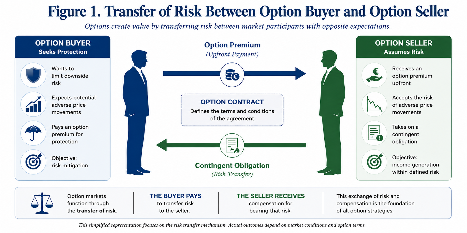
Figure 1. Transfer of Risk Between Option Buyer and Option Seller

Figure 1. Options transfer market risk between two counterparties with fundamentally different expectations. Whilst the buyer acquires protection against adverse price movements, the seller receives an option premium in exchange for assuming the corresponding contingent obligation. This transfer of risk constitutes the economic foundation upon which option markets operate and explains the central role played by option premiums in systematic short-put strategies.

The following sections revisit the theoretical foundations of implied volatility before examining why market observations systematically depart from the assumptions of constant volatility. Attention is subsequently devoted to the informational content embedded within volatility skews and smiles, leading to the introduction of a practical analytical framework intended to investigate whether changes in the implied volatility surface may contribute to the identification of favourable environments for systematic cash-secured put-selling.

The Black-Scholes-Merton Framework: An Elegant Model Built upon Simplifying Assumptions

Since its publication in 1973, the Black-Scholes-Merton model has become one of the most influential achievements in financial economics. Beyond providing a closed-form solution for the valuation of European options, it established a rigorous mathematical framework linking derivative prices to the stochastic behaviour of the underlying asset. More than half a century later, despite the emergence of increasingly sophisticated numerical models, Black-Scholes remains the common language of option markets.

Its enduring success stems from the remarkable intuition underlying the model. Rather than attempting to forecast future prices directly, Black-Scholes demonstrates that an option may be replicated through a continuously adjusted portfolio combining the underlying asset and a risk-free investment. Under a specific set of assumptions, this replication argument leads to a unique theoretical option value independent of investors’ individual expectations.

These assumptions are well known. Asset prices are assumed to follow a geometric Brownian motion with constant volatility. Markets are perfectly liquid and frictionless, allowing continuous trading without transaction costs or taxes. Interest rates remain constant throughout the life of the contract, whilst European options can only be exercised at maturity. Finally, market participants are assumed to behave rationally and possess homogeneous expectations.

From a practical perspective, few of these assumptions are fully satisfied in real financial markets. Transaction costs exist, volatility varies continuously, liquidity fluctuates and investors frequently react in heterogeneous ways to new information. Nevertheless, the model remains extraordinarily useful because it provides a coherent reference framework from which market observations may subsequently be interpreted.

One of its most significant contributions lies in the concept of implied volatility. Rather than treating volatility as an observable market variable, the Black-Scholes equation can be solved inversely. By inserting the observed option premium together with the remaining market parameters, it becomes possible to determine the level of volatility required for the theoretical model to reproduce the market price exactly. This inferred quantity is known as implied volatility.

Implied volatility therefore represents considerably more than a simple mathematical parameter. It embodies the level of uncertainty collectively embedded within option prices by market participants. Every quoted option premium implicitly reflects the market’s assessment of future price variability, making implied volatility one of the most informative indicators available to option traders.

Yet an important observation immediately follows. If the assumptions of the Black-Scholes model were perfectly satisfied, every option sharing the same maturity would exhibit the same implied volatility, irrespective of its strike price. Reality tells a rather different story.

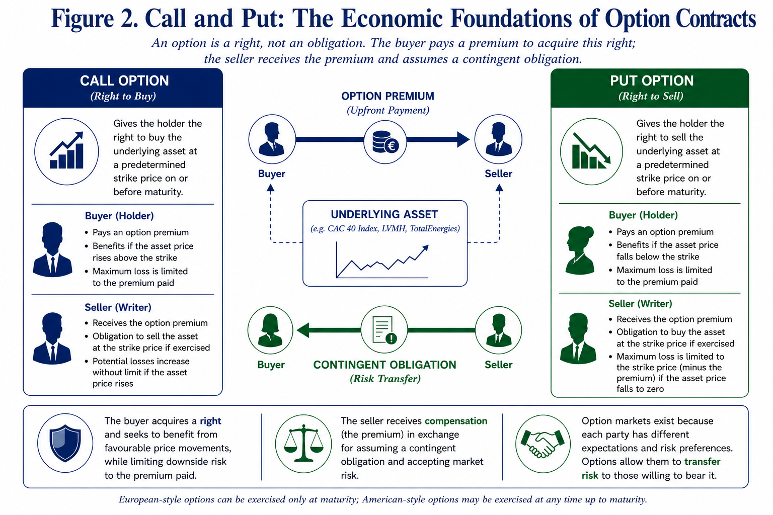
Figure 2. Call and Put: The Economic Foundations of Option Contracts

Figure 2. A call option grants its holder the right, but not the obligation, to purchase the underlying asset at a predetermined strike price. Conversely, a put option grants the right to sell the underlying asset under identical contractual conditions. In both cases, the buyer acquires a right by paying an option premium, whilst the seller receives that premium in exchange for assuming the corresponding contingent obligation.

Implied volatility: From a Single Parameter to a Market Indicator

The original formulation of Black-Scholes implicitly assumes that volatility constitutes a characteristic of the underlying asset itself. If this were strictly true, every option written on the same asset and sharing an identical maturity would produce the same implied volatility once observed market prices are introduced into the valuation equation.

Empirical evidence has demonstrated otherwise. When implied volatilities are computed across a range of strike prices, they rarely remain constant. Instead, they exhibit systematic patterns whose shape varies according to both the underlying asset and prevailing market conditions. These observations, initially regarded as anomalies, have gradually become recognised as fundamental characteristics of option markets. The discrepancy is not accidental. It reflects the collective behaviour of investors rather than any mathematical imperfection within the pricing equation itself.

Institutional investors, pension funds and asset managers frequently purchase out-of-the-money put options to protect equity portfolios against severe market declines. This persistent demand for downside insurance increases put premiums relative to those predicted under constant volatility assumptions. Consequently, implied volatilities extracted from these option prices become progressively higher as strike prices decrease.

The resulting asymmetry gives rise to what practitioners commonly describe as the volatility skew. Rather than representing a flaw in Black-Scholes, the skew reveals how financial markets collectively price extreme downside events. It therefore provides direct insight into investors’ perception of risk, their appetite for protection and the relative scarcity of option sellers willing to assume such exposure.

Viewed from this perspective, implied volatility ceases to be merely an intermediate calculation. It becomes a market variable, capable of conveying valuable information regarding the balance between fear and confidence prevailing amongst market participants.

From the Volatility smile to the Volatility skew

When implied volatilities are calculated across a range of strike prices for a given maturity, the resulting profile rarely corresponds to the horizontal line predicted by the Black-Scholes-Merton model. Instead, distinct empirical patterns emerge according to both the underlying asset and prevailing market conditions.

The earliest observations concerned currency and commodity options, where implied volatility frequently followed a symmetrical U-shaped profile. Deep in-the-money and deep out-of-the-money options exhibited higher implied volatilities than contracts whose strike prices were close to the prevailing market price. This phenomenon rapidly became known as the volatility smile, reflecting the characteristic curvature obtained when implied volatilities were plotted against strike prices.

The market crash of October 1987 marked a decisive turning point in option pricing. Following the unprecedented decline in global equity markets, practitioners observed that the Black-Scholes-Merton assumption of constant volatility no longer matched market prices. Implied volatilities began to differ substantially across strike prices, particularly for downside put options, reflecting investors’ increased demand for protection against extreme losses. Rather than attempting to force market prices into a single volatility parameter, traders progressively adopted the implied volatility surface itself as the practical input for option valuation. Since then, the smile and, even more prominently, the volatility skew have become standard features of option markets and indispensable tools for pricing, hedging and risk management.

Although initially regarded as an anomaly, the volatility smile gradually became recognised as a natural consequence of market behaviour rather than a failure of financial theory. Financial returns do not follow the perfectly lognormal distribution assumed by the Black-Scholes-Merton framework. Instead, empirical distributions exhibit heavier tails, occasional jumps and varying degrees of asymmetry, all of which contribute to systematic differences in implied volatility across strike prices.

Equity index options, however, generally display a markedly different pattern. Rather than producing a symmetrical smile, implied volatility typically increases as strike prices decrease. Conversely, call options with higher strike prices tend to exhibit progressively lower implied volatilities. The resulting profile no longer resembles a smile but rather a downward-sloping curve commonly referred to as the volatility skew.

This asymmetry is far from accidental. It reflects the structural demand for downside protection that characterises modern equity markets. Pension funds, insurance companies, institutional asset managers and other long-term investors regularly purchase out-of-the-money put options to protect diversified equity portfolios against severe market downturns. Such contracts effectively operate as insurance policies against extreme market events.

As demand for these protective puts increases, their market prices rise beyond the levels predicted by constant-volatility models. Once these prices are translated back into implied volatilities through the Black-Scholes equation, lower strike prices systematically exhibit higher implied volatility. The volatility skew therefore represents considerably more than a graphical curiosity. It provides a direct visual representation of how financial markets collectively price downside risk.

Rather than indicating that the Black-Scholes model has failed, the skew demonstrates that investors attribute different probabilities to upward and downward market movements. In practice, the cost of insuring against a sharp decline is significantly greater than the cost of participating in an equally pronounced upward movement. For option sellers, this distinction is of particular importance.

The additional premium associated with out-of-the-money put options constitutes the primary source of return for many systematic short-put strategies. Yet this additional premium simultaneously reflects the market’s perception of elevated downside risk. The option seller is therefore continuously confronted with a fundamental trade-off: richer premiums are generally accompanied by greater uncertainty.

Understanding this relationship represents the first step towards interpreting implied volatility not merely as a pricing parameter, but as a genuine source of market information.

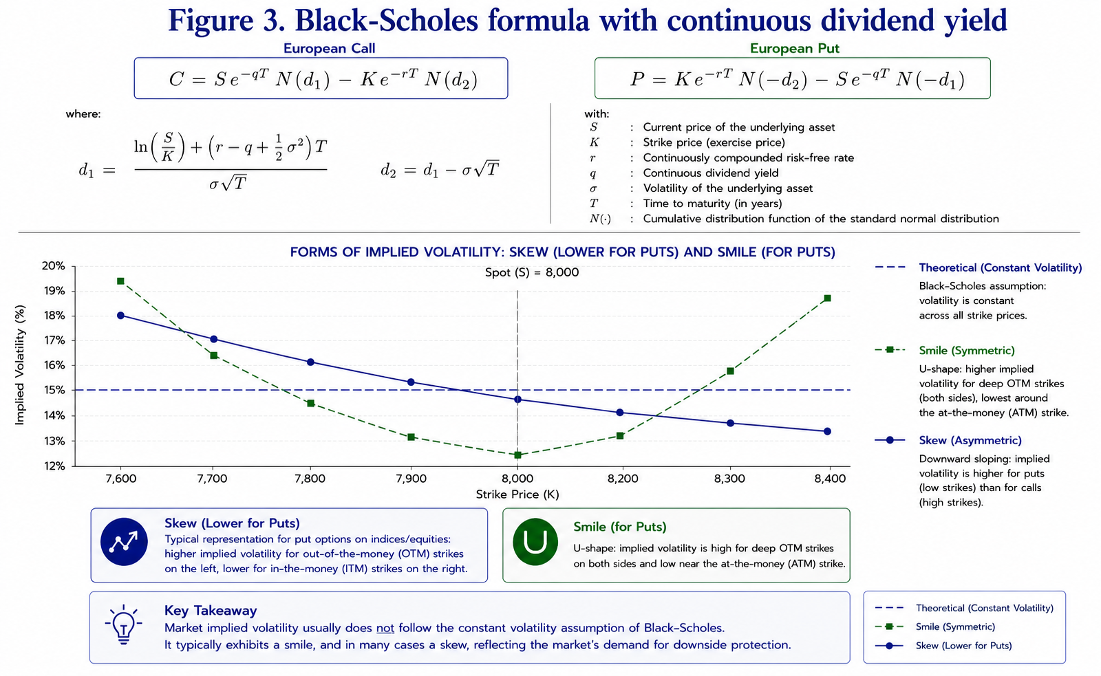
Figure 3. Black-Scholes-Merton Model with Continuous Dividend Yield

Figure 3. Under the Black-Scholes assumption of constant volatility, implied volatility should remain identical across strike prices. Empirical observations reveal two distinct market structures: the volatility smile, historically observed in several currency option markets, and the downward volatility skew that characterises most equity index options.

The Volatility skew as a Measure of Collective Risk Perception

Traditional option pricing theory treats implied volatility as a parameter required to value derivative contracts. Market practitioners increasingly adopt a rather different perspective. For many traders, implied volatility has progressively become an observable market variable.

Its level reflects the price investors collectively assign to uncertainty, whilst its distribution across strike prices reveals how that uncertainty is allocated between favourable and unfavourable market scenarios. This distinction is fundamental.

If all future price movements were regarded as equally probable, the volatility surface would remain broadly symmetrical. The persistent existence of a downward skew instead demonstrates that investors consistently attribute a greater economic significance to adverse market movements than to equivalent upward fluctuations. In this respect, the volatility skew may be interpreted as a continuously updated measure of collective risk aversion.

Unlike conventional market indicators, which frequently rely upon historical observations, implied volatility incorporates forward-looking expectations embedded directly within option prices. Every transaction reflects the judgement of buyers and sellers regarding future uncertainty. The resulting volatility surface therefore aggregates thousands of independent market assessments into a single observable structure. From the perspective of a systematic put seller, the implications are immediate.

Periods during which the skew becomes exceptionally steep frequently coincide with heightened demand for downside protection. Conversely, a gradual flattening of the skew may indicate that the market is beginning to reassess the likelihood of extreme adverse scenarios.

The central hypothesis explored throughout the remainder of this article is based precisely upon this observation. Rather than considering implied volatility in isolation, greater attention may usefully be devoted to the evolution of the entire volatility surface.

Looking Beyond Implied volatility: Can the Volatility surface Become a Decision-Support Tool?

For most option practitioners, implied volatility is primarily regarded as a pricing variable. Whether calculated directly from market quotations or displayed by professional trading platforms, it is generally interpreted as a measure of the market’s expectation of future uncertainty. Consequently, trading decisions often rely upon a relatively simple observation: higher implied volatility produces higher option premiums.

For investors writing cash-secured puts, this relationship is naturally attractive. Selling options during periods of elevated implied volatility allows the collection of larger premiums whilst maintaining identical contractual obligations. Yet this apparent advantage immediately raises a practical difficulty.

Periods characterised by elevated implied volatility rarely occur in isolation. They are frequently associated with deteriorating market sentiment, increasing downside risk and heightened investor demand for protection. In such circumstances, high option premiums merely compensate sellers for assuming substantially greater uncertainty. The absolute level of implied volatility therefore provides only a partial description of market conditions. A more informative question may instead concern the behaviour of implied volatility itself.

Is the volatility surface continuing to steepen? Has it reached a plateau? Or has it begun to return progressively towards more stable market conditions?

These questions introduce an important distinction between two different approaches to option selling. The first consists simply of identifying expensive options based on their implied volatility. The second seeks to determine whether market conditions themselves have begun to evolve in favour of the option seller. The distinction is subtle but potentially significant.

A market characterised by high implied volatility, and an increasingly steep volatility skew reflects persistent demand for downside protection. Under such circumstances, option premiums may continue to increase despite already appearing historically elevated.

Conversely, if implied volatility remains relatively high whilst the overall structure of the volatility surface begins to normalise, market expectations may be undergoing a gradual transition. Although uncertainty remains elevated, the balance between buyers and sellers of protection may already be changing.

From the perspective of a systematic option seller, such an environment appears fundamentally different. The option premium remains attractive, yet the dynamics of market expectations may already be evolving towards greater stability. This observation forms the central hypothesis explored in the present work.

Rather than evaluating implied volatility solely through its absolute level, the proposed approach investigates whether the progressive normalisation of the implied volatility surface may itself constitute useful information capable of assisting the timing of cash-secured short put strategies.

Importantly, this hypothesis should not be interpreted as an attempt to forecast future market prices. No volatility model can predict future market movements with certainty. Instead, the objective is considerably more modest.

The purpose is to investigate whether the collective information continuously embedded within option prices can be organised into a coherent analytical framework capable of improving the selection of favourable option-selling environments.

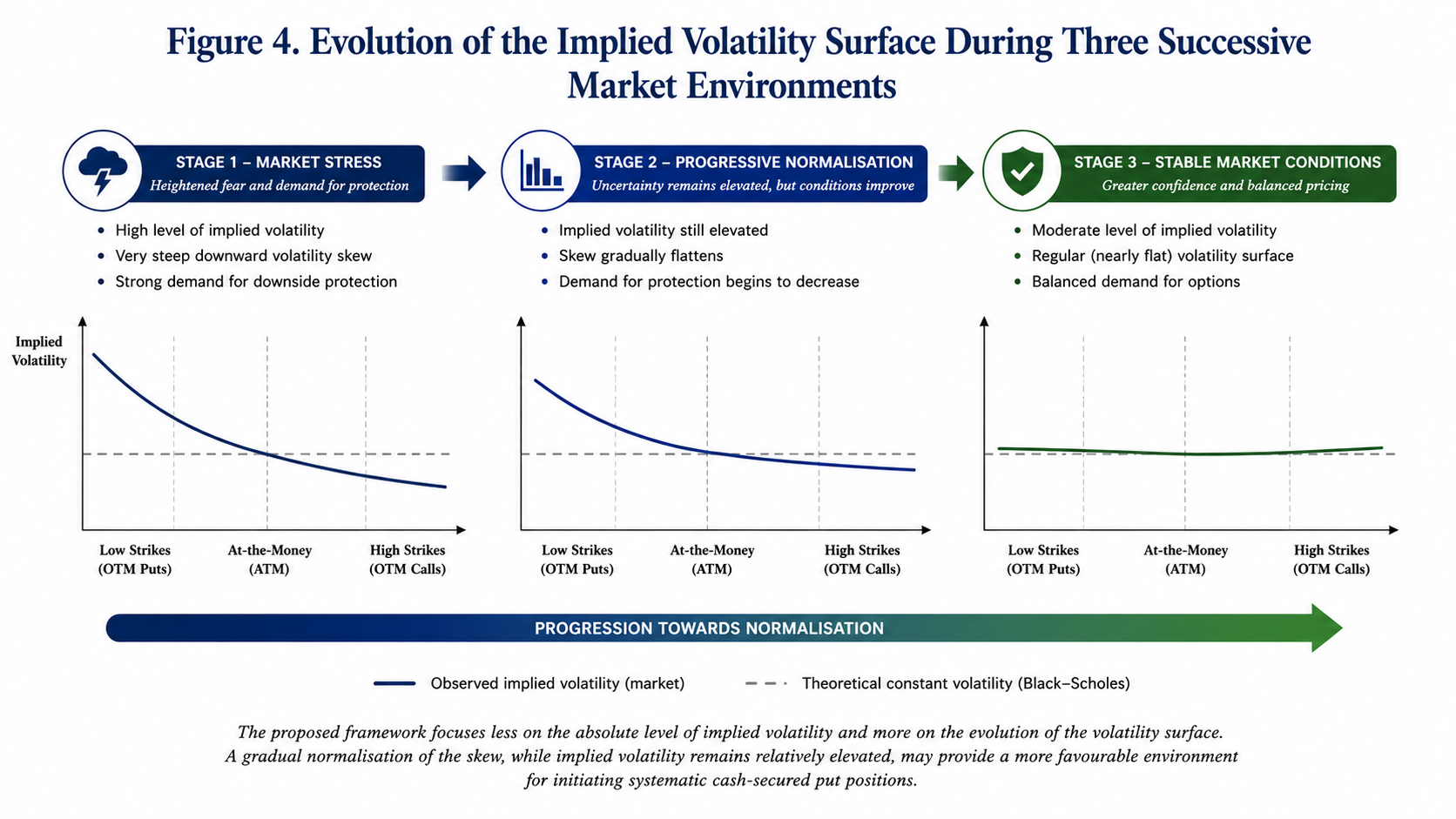
Three Market Environments for Systematic Put Selling

Figure 4. The proposed framework focuses less on the absolute level of implied volatility than on the evolution of the volatility surface itself. A gradual normalisation of the skew whilst option premiums remain comparatively elevated may provide a more favourable environment for initiating systematic cash-secured put positions.

Towards a Decision-Support Framework Based on Volatility surface Dynamics

The preceding discussion naturally raises a practical question: if the geometry of the implied volatility surface reflects the collective assessment of market risk, can its evolution also provide useful information regarding the timing of option-selling strategies?

This question forms the starting point of the present investigation. Rather than considering implied volatility as a static variable observed at a single point in time, the proposed framework examines the volatility surface as a dynamic structure whose characteristics evolve continuously in response to changing market expectations. The distinction is important.

Most market participants focus primarily on the absolute level of implied volatility. Elevated implied volatility is generally interpreted as an opportunity to collect richer option premiums, whilst low implied volatility often discourages option-selling strategies. Such reasoning, however, overlooks an essential aspect of market behaviour.

Two market environments may exhibit comparable average implied volatilities whilst reflecting fundamentally different underlying conditions.

In the first case, implied volatility may still be increasing, accompanied by a progressively steeper volatility skew and a persistent demand for downside protection. In the second, implied volatility may remain elevated, but the volatility surface itself may already be beginning to stabilise, suggesting that market participants are gradually reassessing the probability of extreme downside events.

From the perspective of a systematic put seller, these two situations should not necessarily be regarded as equivalent. Although option premiums may appear imilarly attractive, the evolution of collective market expectations differs substantially.

The working hypothesis explored throughout this study is therefore deliberately modest. Rather than attempting to predict future market prices, the objective is to determine whether the progressive normalisation of the implied volatility surface may provide additional information capable of assisting the selection of favourable market environments for initiating cash-secured short put positions.

In this respect, the volatility surface is not viewed as a forecasting instrument. Instead, it is interpreted as a continuously updated representation of market sentiment whose evolution may contribute to a more disciplined investment process.

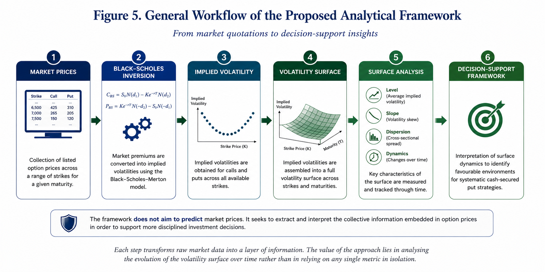
Decision-Support Framework

Figure 5. General workflow of the proposed analytical framework. Market option prices are first converted into implied volatilities using the Black-Scholes-Merton model. The resulting volatility surface is subsequently analysed through a series of descriptive indicators before being interpreted within a decision-support framework for systematic cash-secured put strategies.

Methodological Approach

The methodology developed in this work follows a sequence of analytical steps intended to transform raw market quotations into interpretable market indicators.

The process begins with the systematic collection of listed option prices for a given underlying asset and maturity. Preference is given to highly liquid option contracts to minimise distortions resulting from wide bid-ask spreads or infrequent trading activity.

Observed market premiums are then converted into implied volatilities through the inverse application of the Black-Scholes-Merton pricing equation. Once computed across the available strike prices, these implied volatilities collectively define the observed volatility surface for the selected maturity.

Rather than analysing each implied volatility independently, several global characteristics of the surface are examined simultaneously.

Attention is devoted to:

the overall level of implied volatility;
the slope of the volatility skew;
the degree of cross-sectional dispersion across strike prices;
the temporal evolution of these characteristics between successive market observations.

The purpose of this multidimensional approach is to characterise market conditions more comprehensively than would be possible through the observation of implied volatility alone. Naturally, not all option markets exhibit comparable behaviour.

The preliminary investigations presented in this article suggest that market liquidity and option maturity play a decisive role in determining the regularity of the resulting volatility surface. Highly liquid equity index options with medium- to long-term maturities appear particularly well suited to this type of analysis, whereas shorter maturities or less actively traded underlying assets may generate substantially noisier implied volatility structures.

These observations should not be interpreted as definitive conclusions. Rather, they provide an empirical motivation for the exploratory analyses presented in the following section.

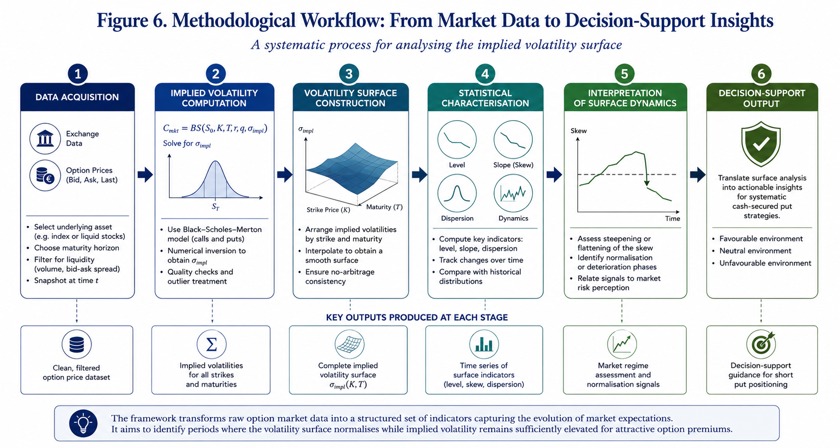
Methodological Approach

Figure 6. Illustrative workflow describing the successive stages of the proposed methodology: market data acquisition, implied volatility computation, volatility surface construction, statistical charac-terisation and decision-support interpretation.

Preliminary Empirical Observations

The analytical framework presented above was subsequently applied to listed option data to examine whether the proposed interpretation of the implied volatility surface could be observed under actual market conditions.

At this stage, the objective was not to perform an exhaustive statistical validation of the methodology. Rather, the purpose was to investigate whether the dynamics of the implied volatility surface exhibited sufficiently regular behaviour to justify further quantitative analysis.

Several option chains were therefore examined, covering different underlying assets and maturities.

Attention was devoted to the CAC 40 index, whose option market offers a high level of liquidity across a broad range of strike prices. Additional observations were conducted on selected individual equities to assess the robustness of the approach under different market conditions.

The first observation concerns the influence of option maturity.

Short-dated options, particularly those approaching expiration, frequently generated irregular implied volatility profiles. Individual quotations occasionally produced local distortions, whilst relatively small pricing discrepancies resulted in disproportionately large variations in calculated implied volatility. Such behaviour appears consistent with the increasing influence of time decay and the reduced amount of remaining time value as maturity approaches.

Consequently, short maturities should be interpreted with caution when constructing continuous volatility surfaces. A markedly different picture emerged for longer maturities.

Options with approximately six months to one year remaining until expiration generally produced substantially smoother implied volatility structures. The resulting volatility skews exhibited the regular downward slope commonly described in the empirical literature, with only limited local distortions across neighbouring strike prices.

These observations proved particularly apparent for the CAC 40 index.

The high liquidity of the option market appeared to facilitate a more stable estimation of implied volatility, thereby providing a significantly more coherent representation of the underlying volatility surface. An equally important observation concerns the distinction between index options and individual equity options.

Whilst the CAC 40 generated relatively stable and interpretable volatility structures, several individual equities produced substantially noisier results. In certain cases, isolated market quotations generated implausibly high or even negative implied volatility estimates, suggesting either temporary pricing inconsistencies or insufficient market liquidity.

Such observations reinforce an important practical consideration.

The proposed methodology appears particularly well suited to highly liquid option markets where quoted premiums reflect continuous interaction between buyers and sellers. Conversely, less liquid markets may introduce local pricing distortions capable of obscuring the global characteristics of the volatility surface.

These preliminary observations do not constitute definitive statistical conclusions.

Nevertheless, they suggest that both liquidity and maturity represent essential prerequisites when analysing implied volatility surfaces for decision-support purposes.

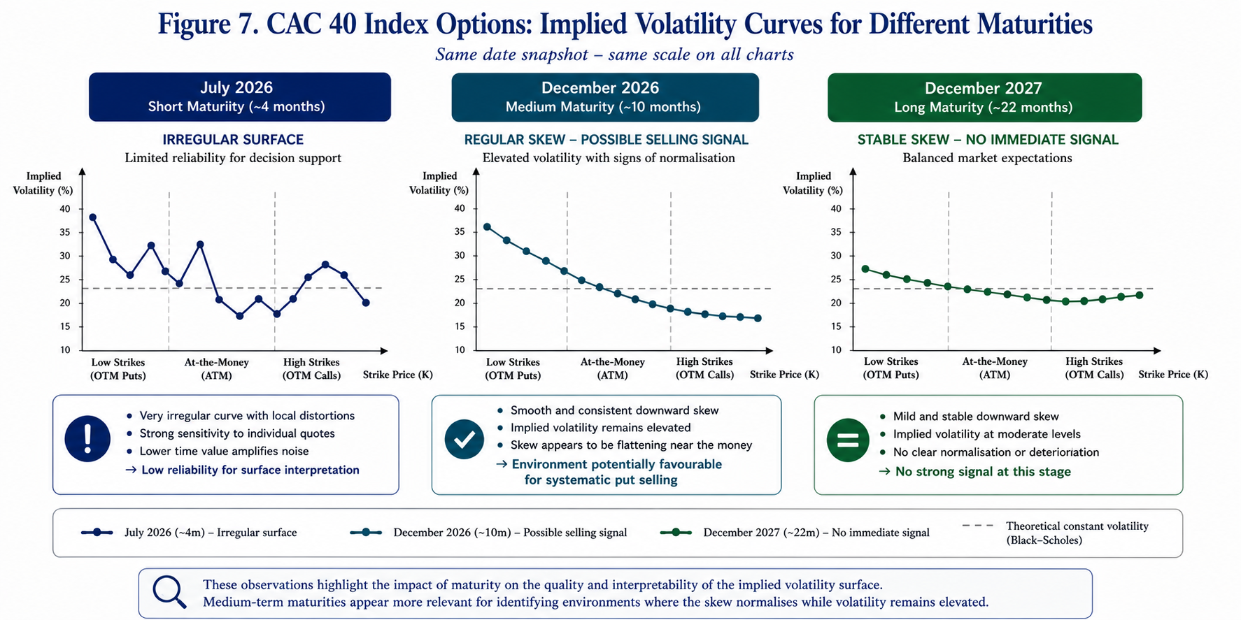
Implied Volatility Curves

Figure 7. Comparison of implied volatility curves obtained for different maturities. Short-dated maturities frequently exhibit irregular local behaviour owing to limited time value and increased pricing sensitivity. Longer maturities generally produce smoother volatility skews, thereby facilitating the interpretation of surface dynamics.

A further observation emerged during the analysis: although several volatility surfaces displayed the expected downward skew, not all of them generated identical decision-support signals.

Certain maturities exhibited a progressive flattening of the skew whilst implied volatility remained at comparatively elevated levels. Others retained a persistent steep slope despite similar average volatility levels. This distinction proved particularly informative. If confirmed through broader empirical investigation, it suggests that the overall geometry of the volatility surface may contain additional information beyond the absolute level of implied volatility alone. From the perspective of systematic option selling, this observation may prove significant.

A market characterised by elevated implied volatility, and a progressively normalising volatility surface appears fundamentally different from one in which both implied volatility and downside protection demand continue to increase simultaneously.

The former may correspond to a market gradually returning towards equilibrium. The latter may still reflect an environment dominated by uncertainty.

Consequently, analysing the dynamics of the volatility surface rather than its static characteristics alone may provide a richer description of prevailing market conditions.

The following section illustrates how these observations may be translated into a practical decision-support framework for systematic cash-secured put strategies.

Discussion

The preliminary observations presented above suggest that the practical usefulness of the implied volatility surface depends upon two essential conditions: the quality of market data and the maturity of the option contracts under consideration.

The first point appears relatively intuitive.

Implied volatility is not directly observable. It is inferred from quoted option prices through the inverse application of the Black-Scholes-Merton model. Consequently, any inconsistency in market quotations is immediately reflected in the calculated implied volatilities.

This phenomenon proved particularly evident during the exploratory analyses conducted on individual equities.

Whilst certain option chains generated coherent volatility structures, others produced isolated implied volatility values that were incompatible with neighbouring strike prices. In a limited number of cases, implausible or unstable implied volatility estimates were obtained despite apparently valid market quotations. Such behaviour most likely reflects temporary liquidity deficiencies, unusually wide bid-ask spreads or isolated transactions executed outside normal market conditions.

These observations underline an important methodological requirement.

The proposed framework should preferably be applied to option markets characterised by sufficient liquidity and a broad distribution of actively traded strike prices. Under such conditions, quoted premiums are more likely to represent the consensus valuation of market participants rather than isolated transactions.

The second observation concerns option maturity.

Short-dated contracts frequently produced irregular volatility profiles whose local fluctuations appeared dominated by pricing noise rather than genuine changes in market expectations. As expiration approaches, the remaining time value becomes progressively smaller, and option prices exhibit increasing sensitivity to relatively minor changes in the underlying asset. Consequently, the resulting implied volatility estimates become substantially less stable.

Conversely, medium- and long-dated maturities generally generated considerably smoother volatility structures.

The downward skew remained clearly identifiable whilst local distortions became significantly less pronounced. This regularity considerably facilitated the interpretation of the surface and its evolution over successive market observations.

Among the datasets examined, listed CAC 40 index options consistently provided the most coherent results. Their combination of high liquidity, narrow bid-ask spreads and broad strike availability produced volatility surfaces whose overall geometry remained remarkably stable. This characteristic makes such instruments particularly well suited to exploratory research concerning the dynamics of implied volatility.

An additional observation deserves particular attention: not every regular volatility surface generated the same analytical conclusion.

Certain maturities displayed a progressive flattening of the volatility skew whilst implied volatility remained comparatively elevated. Others retained a persistent and pronounced downward slope despite exhibiting similar average volatility levels. This distinction appears especially interesting.

If future empirical analyses confirm these preliminary observations, the evolution of the volatility surface may provide information that cannot be obtained from the absolute level of implied volatility alone. Such a conclusion would carry practical implications for systematic option-selling strategies.

Rather than selecting opportunities exclusively according to premium levels or historical volatility, investors may benefit from incorporating the dynamics of the implied volatility surface into their broader decision-making process. Naturally, these findings should be interpreted with appropriate caution.

The present work remains exploratory in nature and does not claim to establish a predictive model. Instead, it proposes an analytical framework intended to organise market information already embedded within option prices into a more coherent decision-support process.

Further empirical investigation involving longer observation periods, multiple market regimes and additional underlying assets will naturally be required before more general conclusions may be drawn.

Evolution of the Implied Volatility Surface

Figure 8. Evolution of the implied volatility surface across successive market observations. The figure illustrates the conceptual distinction between a market in which the volatility skew continues to steepen and one in which the surface progressively normalises whilst implied volatility remains comparatively elevated.

Practical Implications for Systematic Put Sellers

From a practical perspective, the observations discussed throughout this article suggest that implied volatility should perhaps be interpreted less as an isolated numerical indicator and more as one component of a broader analytical framework.

Option sellers have traditionally focused on premium maximisation. Although this objective remains entirely legitimate, premium alone provides only a partial description of prevailing market conditions.

The same premium may arise under markedly different market environments. One may correspond to an increasingly stressed market characterised by rapidly rising demand for downside protection. Another may reflect a market in which uncertainty remains elevated but has already begun to stabilise.

Distinguishing between these situations may prove particularly valuable when implementing systematic cash-secured put strategies. Rather than attempting to forecast market direction, the proposed framework encourages a more disciplined interpretation of the information continuously embedded within option prices.

In this respect, the implied volatility surface becomes considerably more than a graphical representation of option quotations. It evolves into a dynamic indicator describing the collective perception of risk within financial markets.

Conclusion

The Black-Scholes-Merton model remains the fundamental reference upon which modern option pricing is built. Although one of its central assumptions — constant volatility — is systematically contradicted by market observations, these apparent discrepancies have progressively become one of the richest sources of information available to option practitioners.

The implied volatility surface should therefore not merely be regarded as a technical consequence of option pricing theory. It reflects the collective judgement of market participants regarding future uncertainty, the asymmetrical pricing of downside risk and the continuously evolving balance between buyers and sellers of financial protection. The purpose of the present study has been to explore whether this information may be exploited beyond its traditional pricing function.

Rather than concentrating exclusively on the absolute level of implied volatility, this article has proposed a broader analytical perspective based upon the dynamics of the entire volatility surface. Attention has been devoted to the progressive evolution of the volatility skew, whose gradual normalisation may provide additional insight into changing market conditions.

The preliminary empirical observations presented throughout this paper suggest practical conclusions.

First, market liquidity appears to constitute a fundamental prerequisite for obtaining sufficiently stable implied volatility surfaces. Highly liquid option markets, such as listed CAC 40 index options, produce considerably more coherent structures than many individual equity options, whose implied volatilities may occasionally be distorted by isolated transactions or limited trading activity.

Secondly, option maturity also plays a decisive role. Medium- and long-dated contracts generally generate smoother volatility surfaces that appear more suitable for structural analysis than very short-dated maturities, where the increasing influence of time decay frequently introduces substantial local irregularities.

Finally, and perhaps most importantly, the observations suggest that two markets exhibiting comparable average implied volatility levels may nevertheless convey markedly different information through the geometry of their respective volatility surfaces. This distinction may prove particularly relevant for systematic cash-secured put strategies.

Whilst elevated implied volatility undoubtedly increases option premiums, the progressive normalisation of the volatility surface may provide complementary information regarding the evolution of collective market expectations. The proposed framework should therefore not be interpreted as a predictive model. Financial markets remain inherently uncertain, and no analytical methodology can eliminate investment risk.

Instead, the approach presented here seeks to organise information already embedded within option prices into a structured decision-support framework capable of complementing more traditional valuation techniques. Viewed from this perspective, the implied volatility surface ceases to be merely a graphical representation of option prices. It becomes a dynamic description of market behaviour.

Understanding how this structure evolves through time may ultimately prove as informative as measuring its absolute level at any single observation date.

Limitations and Future Research

The present study should be regarded as an exploratory investigation rather than a definitive empirical validation. Several limitations naturally remain.

The observations reported here are based upon a limited number of underlying assets and observation dates. Broader empirical investigations covering multiple market regimes, longer historical periods and additional asset classes will be required before more general conclusions may be established. Future research could also investigate whether quantitative indicators describing the geometry of the implied volatility surface — such as skew slope, local curvature or cross-sectional dispersion — may be systematically incorporated into algorithmic decision-support models for option-selling strategies.

Another promising avenue concerns the comparative behaviour of implied volatility surfaces across different asset classes, including equity indices, individual equities, exchange-traded funds and commodity options.

Finally, machine learning techniques may eventually provide complementary tools capable of identifying recurring patterns within the evolution of volatility surfaces. Such approaches, however, should be viewed as extensions of the present analytical framework rather than substitutes for the economic interpretation of market behaviour. Ultimately, the principal contribution of this work lies less in proposing a new pricing model than in suggesting an alternative way of interpreting information already contained within option markets. If the geometry of the implied volatility surface indeed reflects the collective perception of financial risk, then monitoring its evolution may offer valuable additional insight into the timing of systematic option-selling strategies.

Download the Summary Infographic

Readers wishing to retain a concise visual summary of the concepts presented throughout this article may download the accompanying high-resolution infographic below.

Download the Summary Infographic (High-Resolution PDF)

Useful resources

Black, F., & Scholes, M. (1973). The Pricing of Options and Corporate Liabilities. Journal of Political Economy, 81(3), 637-654.

Gatheral, J. (2006). The Volatility Surface: A Practitioner’s Guide. John Wiley & Sons.

Hull, J. C. (2024). Options, Futures and Other Derivatives (11th ed.). Pearson.

Merton, R. C. (1973). Theory of Rational Option Pricing. The Bell Journal of Economics and Management Science, 4(1), 141-183.

Natenberg, S. (2015). Option Volatility and Pricing (2nd ed.). McGraw-Hill Education.

Rebonato, R. (2004). Volatility and Correlation: The Perfect Hedger and the Fox. John Wiley & Sons.

Taleb, N. N. (1997). Dynamic Hedging: Managing Vanilla and Exotic Options. John Wiley & Sons.

About the Author

Tis article was written in July 2026 by Frédéric VALOGNES , who is a lecturer in corporate finance, financial analysis, financial markets and derivatives, with more than twenty-five years of professional experience spanning financial management, higher education, research administration and executive training. He is a Certified European Financial Analyst (CEFA®), a professional designation awarded by the European Federation of Financial Analysts Societies (EFFAS), Frankfurt.

Author’s Note

This article is intended solely for educational and research purposes. It presents the author’s personal reflections on implied volatility, option pricing and systematic option-selling strategies. It should not be construed as investment advice or as a recommendation regarding any financial instrument or trading strategy.

The ideas developed in this article are the result of many years of teaching, professional practice and ongoing research in corporate finance, financial analysis, financial markets and derivatives. They have also been enriched by numerous discussions with academics, finance professionals and market practitioners, whose expertise, critical insights and constructive exchanges have played an important role in shaping the analytical framework presented here.

The author wishes to express his sincere gratitude to all those who have contributed, directly or indirectly, to the development of these ideas. Their encouragement, intellectual generosity and commitment to rigorous financial analysis have been a constant source of inspiration.

Implied Volatility Surface: Smiles, Smirks and Term Structure

July 17, 2026June 29, 2026 by Saral BINDAL

In this article, Saral BINDAL (Indian Institute of Technology Kharagpur, Metallurgical and Materials Engineering, 2024-2028 & Research assistant at ESSEC Business School) explains the implied volatility surface: its characteristic shapes, static arbitrage constraints, and application using S&P 500 index options data.

Introduction

In financial markets characterized by uncertainty, volatility is a crucial factor in the valuation of derivative securities. For options traders, an option price is essentially volatility. Although options are traded at monetary prices, professionals routinely quote and compare them in terms of implied volatility (%), making volatility the common language of options markets. Moreover, in a reverse way, implied volatility occupies a central role as a forward-looking indicator that reflects the market’s expectations of future price fluctuations embedded in option prices.

Under the Black-Scholes-Merton (BSM) model, volatility is assumed to be constant and independent of option characteristics like the strike price (K) and the time to maturity (T). Empirical evidence, however, reveals that implied volatility varies across option contracts and especially depends on both parameters K and T of the option.

Implied volatility curves: the strike dimension

Volatility curves represent a cross-sectional view of the implied volatility surface (IVS), depicting the relationship between implied volatility and strike price for a fixed maturity. They are constructed by plotting implied volatility as a function of strike while holding time-to-maturity constant.

The volatility curves are commonly observed in two distinct shapes, most notably the volatility smile and the volatility smirk. A detailed discussion of the empirical relationship between implied volatility and option moneyness, the associated stylized facts, and their economic interpretation can be found in the article Volatility curves: smiles and smirks.

Figure 1 below illustrates the implied volatility smile (1a) and smirk (1b).

Figure 1a and 1b. Implied Volatility Smile and Smirk
Implied Volatility Curves (smile and smirk)
Source: computation by the author (with python).

Term structure of implied volatility: the maturity dimension

While volatility curves describe the strike dependence of implied volatility, the maturity dimension captures how implied volatility varies across expiration dates for a given strike. This relationship is commonly referred to as the term structure of implied volatility.

Using daily implied volatility data for S&P 100 index options (December 1983 to September 1987), Stein (1989) documented that volatility shocks are transmitted across maturities more strongly than predicted by standard rational expectations theory. Under this standard theoretical framework, because implied volatility is strongly mean-reverting, a near-term shock should naturally decay over time, causing long-dated implied volatilities to change by only a fractional amount. However, following an increase in short-dated implied volatility, long-dated implied volatilities tend to rise by a disproportionately large amount, indicating that changes in near-term uncertainty heavily influence market expectations over a broad range of maturities.

Using data for options on the S&P 500, FTSE 100, DAX 30, CAC 40, and Nikkei 225 stock indexes spanning the period May 9, 1994 to October 12, 2001, Mixon (2007) suggested mean reversion as a key characteristic of the implied volatility term structure. While short-dated implied volatilities exhibit substantial sensitivity to changes in market conditions, long-dated implied volatilities remain comparatively stable, reflecting expectations of convergence toward a long-run volatility level. Consequently, the term structure is generally upward sloping (contango) during periods of low market uncertainty but may become inverted (backwardation) during episodes of market stress, when short-term volatility rises sharply.

Figure 2 illustrates an upward-sloping (2a) and a downward-sloping (2b) implied volatility term structure.

Figure 2a and 2b. Implied Volatility Term Structure

Source: computation by the author (with python).

Christoffersen, Heston, and Jacobs (2009) demonstrate that the volatility term structure is not necessarily monotonic, arguing that capturing its true dynamics requires multifactor stochastic volatility frameworks. Evaluating European S&P 500 call options from 1990 through 2004, their empirical evidence reveals that implied volatility frequently displays significant curvature across maturities. This non-monotonic curvature is difficult to reconcile with traditional single-factor specifications like the benchmark Heston (1993) model, which restricts the term structure of implied volatility because it relies on only a single variance factor to model volatility over time.

Volatility Surface

The volatility surface provides a three-dimensional representation of implied volatility across strike prices and maturities. It is represented by the function σ(K,T), which assigns an implied volatility to each combination of strike price K and time to maturity T that reproduces the observed market option prices under the Black-Scholes-Merton (BSM) model.

Call option price formula under the BSM

Constructed from a cross-section of traded options, the volatility surface provides a comprehensive description of how the market prices uncertainty across both strike price (K) and maturity (T).

Arbitrage constraints

In practice, market option quotes are available only for a discrete set of strikes and maturities. Constructing a continuous volatility surface therefore requires interpolation and smoothing techniques. To ensure economic consistency, we must have σ(K,T) ≥ 0 for all strikes K and expirations T and the resulting surface must satisfy the static no-arbitrage conditions: namely the absence of butterfly arbitrage across strikes and calendar-spread arbitrage across maturities. (see, Breeden & Litzenberger, 1978; Gatheral, 2006)

The absence of butterfly arbitrage requires option prices to remain convex with respect to strike. Equivalently, the risk-neutral probability density implied by option prices must remain non-negative across all strikes, this condition can be expressed as:

Conditon for the absence of butterfly arbitrage

A violation of this condition implies a negative risk-neutral probability density over some range of strikes and leads to arbitrage opportunities.

The absence of calendar-spread arbitrage states that with increase in maturity of an option, it should not result in a reduction of its value, since a longer-dated option provides all the rights of an otherwise identical shorter-dated option together with additional time for favourable price movements to occur. In volatility surface modelling, this condition is typically expressed in terms of the total implied variance

Total implied variance formula

where σ_BS(K,T) denotes the Black-Scholes-Merton implied volatility for strike K and maturity T. Total implied variance measures the total accumulated expected variance over the entire life of the option

For a fixed strike, total implied variance must be non-decreasing with maturity

Conditon for the absence of calendar-spread arbitrage

A violation would imply that a longer-dated option embeds less cumulative uncertainty than a shorter-dated option at the same strike, resulting in an arbitrage opportunity.

Together, the butterfly-arbitrage and calendar-spread-arbitrage constraints ensure that the interpolated volatility surface produces arbitrage-free option prices and a valid risk-neutral distribution.

An Empirical Analysis of the S&P 500 Implied Volatility Surface

In this section, we discuss how an implied volatility surface can be estimated from the S&P 500 index observed market option prices using a parametric model to fit the data and how the parameters can be adjusted to represent different macro-economic stress conditions.

Data collection and filtration

To construct the implied volatility surface, we import the S&P 500 index option chain (set of call and put options across various strikes and maturities) directly from Yahoo! Finance. Because raw market data often contains stale quotes and asynchronous prices, we apply a robust set of filtering techniques to clean the dataset before model estimation.

First, we apply illiquidity filters, removing any option contracts with zero trading volume or zero open interest. Second, we filter the dataset to retain only Out-of-the-Money (OTM) options (OTM puts where K < S₀, and OTM calls where K > S₀). This is a standard practice, as implied volatility is theoretically independent of option type due to Put-Call Parity, focusing strictly on OTM contracts ensures we utilize the most liquid instruments (liquidity being measured by the bid-ask spread) to minimize pricing noise.

Third, we enforce intrinsic value and no-arbitrage boundary conditions. Any contracts with mispriced or economically impossible quotes are filtered out by verifying the upper and lower price bounds for the option contracts as given below

Call and Put option mid-price bounds

where:

K: strike price of the option
S₀: spot price of the underlying asset
T: time to maturity
C: mid-price of a call option
P: mid-price of a put option
r: risk-free rate
q: continuous dividend yield

Finally, we check for vertical (strike) arbitrage to ensure the data adheres to fundamental shape restrictions. We sort the contracts by time-to-maturity and then by strike price in ascending order. We then verify shape monotonicity: for any given maturity, call prices must strictly decrease as the strike price increases, and put prices must strictly increase as the strike price increases. Applying these standard empirical filters ensures a clean, arbitrage-free dataset ready for surface estimation.

Methodology

To model and plot the implied volatility surface as shown below in Figure 1, we implement a parametric approach originally proposed by Dumas, Fleming, and Whaley (1998). This technique fits a deterministic volatility function (DVF) directly through the observed option market data. Under this framework, the implied volatility function is expressed as a second-order polynomial function across log-moneyness (M) and time-to-maturity (T):

DVF Formula

where:

α₀ : Measures the baseline implied volatility level where both log-moneyness and time-to-maturity are equal to zero. Geometrically, this shifts the entire surface straight up or down uniformly
α₁ : Measures the rate of change of volatility across different strikes. Geometrically, this rotates the surface along the moneyness axis, tilting the left wing (puts) up and the right wing (calls) down.
α₂ : Measures the rate of change of the curvature across strikes, defining how sharply the volatility curve bends. Geometrically, this bends the surface into a U-shaped bowl or flattens it into a smooth plane.
α₃ : Measures the rate of change of volatility across the horizon, establishing the slope of the term structure. Geometrically, this tilts the surface front-to-back, altering the premium difference between short-term and long-term contracts.
α₄ : Measures the rate of change of the curvature in the volatility in the term structure across different maturities. Geometrically, this creates a non-linear bend along the time horizon axis.
α₅ : Measures the co-dependency between moneyness and time-to-maturity, modelling how the skew changes as maturity extends. Geometrically, this causes the corners to bend upward or downward simultaneously.

In the polynomial function above, we utilize the log-forward moneyness (M), defined as:

Log-forward moneyness formula

where F₀ is the forward price of the underlying asset, calculated as:

Forward price formula

This is usually done in practice because it is F₀, and not S₀, that represents the expected stock price on the option’s maturity date in a risk-neutral world. Consequently, traders often define an “at-the-money” option as a contract where K = F₀, rather than an option where K = S₀.

To fit this model, we first apply a numerical root-finding algorithm to invert the Black-Scholes-Merton (BSM) pricing model against observed market prices (mid prices defined as the average of bid and ask prices) to extract the market implied volatilities. We restrict our sample to contracts with maturities under one year (T < 1.0) and a log-moneyness of |M| < 0.45. This filters out deep Out-of-the-Money (OTM) options, which typically suffer from low trading volumes and wide bid-ask spreads, as they are primarily held for structural tail-hedging by institutional investors.

Finally, we apply Ordinary Least Squares (OLS) regression to the filtered dataset to solve for the six α parameters simultaneously. Once estimated, these parameters can be used to generate the implied volatility curves, term structures, and 3D surfaces under various macroeconomic stress scenarios, as discussed below.

Empirical Results

Figure 3 illustrates the estimated implied volatility surface of the S&P 500 index using options data collected on June 18, 2026. The market environment at the time of collection was defined by an index spot price (S₀) of $7496.04, a risk-free interest rate (r) of 3.658%, and a continuous dividend yield (q) of 1.04%. Based on these inputs, the resulting empirical surface is presented below.

Figure 3. Implied Volatility Surface of the S&P 500 index options (June 18, 2026)

Source: computation by the author (with python).

From the surface, we can observe that amid ongoing US-Iran tensions in the Middle East, out-of-the-money (OTM) put options exhibit high implied volatility for short-term maturities. This reflects panic buying of downside protection due to fears of conflict escalation and immediate uncertainty in the market. Toward the far end of the maturity, however, the surface balances out with OTM call options. This indicates that while near-term sentiment is dominated by risk aversion, long-term market expectations are highly speculative, positioning for a potential recovery once the geopolitical uncertainty resolves. To isolate and observe these market dynamics more precisely, the individual implied volatility smiles (by strike) and term structures (by maturity) are plotted below.

Figure 4 illustrates the implied volatility curves for three distinct maturities. As discussed above, we can clearly observe the steep downside skew flattening out and transitioning into a asymmetric smile as maturity increases.

Figure 4. Implied Volatility Curves of the S&P 500 options (June 18, 2026)

Source: computation by the author (with python).

Figure 5 illustrates the implied volatility term structure (up to 1 year) for three different strike prices. For out-of-the-money (OTM) call options, we can observe that the term structure is upward-sloping, indicating a long-term uncertainty alongside expectations of an upward market movement. Conversely, the OTM put option term structure is inverted and reflecting high short-term panic and uncertainty. Over the time horizon, this near-term panic subsides, balancing out with the OTM call options in the long run.

Figure 5. Implied Volatility Term Structure of the S&P 500 index options (June 18, 2026)

Source: computation by the author (with python).

The at-the-money (ATM) option term structure exhibits a shallow, non-monotonic U-shape, characterized by elevated short-dated volatility, a flattened middle region, and higher long-term volatility. This reflects that, in the short-to-medium term, the curve demonstrates the classic mean-reversion, where the immediate geopolitical shock dissipates and flattens out over a 3-to-6-month horizon. Conversely, the upward drift at the longer end of the mature horizon reflects the structural term premium demanded by investors to account for broader, open-ended macroeconomic uncertainties, as discussed above in the stylized facts section.

Structural Shifts under Macroeconomic Stress: A Comparative Scenario Analysis

Figure 6 provides a compelling visual framework for observing how the implied volatility surface structurally shifts under different stress conditions. The surface on the left (a) represents the systemic crash caused by the COVID-19 pandemic (2020), while the surface on the right (b) illustrates the hypothetical impact on index options if the ongoing US-Iran conflict were to escalate significantly. These surfaces are constructed by adjusting the values of the six model parameters estimated in the preceding section; as such, they serve as illustrative examples of structural shifts rather than exact numerical forecasts.

Figures 6a and 6b. Implied Volatility Surface of the S&P 500 options under different stress environments

Source: computation by the author (with python).

Note: In both figures, the lightly shaded surface serves as the baseline, representing the actual market implied volatility surface as of June 18, 2026.

From Figure 6a, we can observe a massive surge in overall implied volatility across the board, driven by widespread panic buying of both out-of-the-money (OTM) puts and calls. This systemic shock resulted in a relatively flatter skew but severe inversion across the maturity spectrum, reflecting the acute, immediate fear of economic collapse as global lockdowns were implemented.

In contrast, Figure 6b models a scenario where the US-Iran conflict escalates into a full-scale regional crisis. Such an event would severely disrupt global oil supply chains, acting as a prolonged macroeconomic drag that hits S&P 500 corporate earnings over many months. Because this represents a lingering economic threat rather than an overnight liquidity freeze, the market’s response is highly asymmetric: demand is heavily concentrated in OTM puts for long-term downside protection and a steady increase in long-term implied volatility across the maturity.

While these stress scenarios represent extreme events, day-to-day movements follow structured patterns. Cont and Da Fonseca (2002) showed that daily dynamic deformations of the S&P 500 volatility surface are not chaotic. Instead, using principal component analysis, they demonstrated that surface movements are driven by just a few common statistical factors: parallel shifts, changes in the strike slope (skew), and twists in the maturity curvature.

You can download the Python code provided below, for the construction of the implied volatility curves, term structures and surfaces under different stress conditions as discussed above.

Alternatively, you can download the R code below with the same functionality as in the Python file.

You can download the cleaned S&P 500 index options data for 18 June 2026, as used in the above Python and R codes to make the plots as discussed before.

Volatility Surface Models

A volatility surface determines the risk-neutral distributions implied by option prices (see Option Implied Risk-Neutral Distribution), but it does not uniquely specify the underlying stochastic process governing asset-prices. As highlighted by Cont (2006), this introduces significant model uncertainty: different mathematical frameworks can calibrate perfectly to the exact same market volatility surface today, yet yield wildly divergent prices and hedges for exotic options because they imply different future surface dynamics. Consequently, a substantial body of research has focused on developing models capable of reproducing both the observed shape of the volatility surface and its evolution through time.

The principal modelling approaches include local volatility models, stochastic volatility models, parametric surface models and, more recently, rough volatility models.

Local Volatility Models

In the standard BSM formula, volatility is assumed constant, which however does not correspond to reality, as markets exhibit volatility smile and skews. Local volatility model, extends the BSM, by assuming that volatility is a function of stock price (S_t) and time (t), and the instantaneous local volatility is given by σ_t( S_t,t).

The Dupire (1994) formula that links the instantaneous local volatilities, to the implied volatility surface is given as follows:

Local volatility formula

Stochastic Volatility Models

Stochastic volatility refers to the modelling of volatility using time-dependent stochastic processes, in contrast to the constant volatility assumption made in the standard BSM model. These models are better able to capture the observed features such as volatility clustering and mean reversion. One of the most widely used stochastic volatility models is the Heston (1993) model. The model describes the dynamics of the underlying asset price and its variance using a system of two coupled stochastic differential equations (SDEs), given by:

Stochastic volatility formula

Where:

S_t: is the asset price
v_t: is the instantaneous variance
r: is the risk-free interest rate
q: is the continuous dividend yield
κ: is the speed of mean reversion
θ: is the long-run variance level
σ: is the volatility of variance (volatility-of-volatility)
ρ: is the correlation between shocks to the asset price and variance

Parametric Surface Models

Parametric volatility surface models are used to interpolate and extrapolate implied volatility across strikes and maturities, for sparse or illiquid strikes and ensure the resulting surface is free from static arbitrage (butterfly and calendar arbitrage).

Among the most widely used approaches is the SVI (Stochastic Volatility Inspired) parametrization, developed by Gatheral and Jacquier (2014), which is commonly applied to equity and index volatility surfaces. It models the total implied variance as a function of log-moneyness, providing a parsimonious representation of the volatility smile.

Other important parametric frameworks include the SABR model (Stochastic Alpha, Beta, Rho), which is widely used in interest rate and FX markets, and SSVI (Surface SVI), which extends the SVI framework to ensure arbitrage-free surface dynamics across maturities.

Rough Volatility Models

Rough volatility models represent one of the most important recent developments in volatility modelling. Gatheral, Jaisson, and Rosenbaum (2018) provided the empirical evidence that log-volatility behaves essentially as a fractional Brownian motion with Hurst exponent H of order 0.1, at any reasonable timescale.

The Hurst exponent (H) is a statistical parameter that characterises the roughness of a stochastic process: when H = 0.5, the process reduces to a standard Brownian motion with no memory, corresponding to a random walk. Whereas, values of H > 0.5 indicate persistent behaviour, while H < 0.5 imply anti-persistence, where increments tend to reverse direction more frequently, leading to rougher sample paths.

This observation, led to adoption of the fractional stochastic volatility (FSV) model of Comte and Renault (1998). The Rough FSV (RFSV) in contrast to FSV, is remarkably consistent with ﬁnancial time series data. Compared to classical stochastic volatility models, it better captures the extremely rough nature of volatility paths and enables improved forecasting of realized volatility.

Why should I be interested in this post?

Implied volatility surfaces are among the most important tools in modern quantitative finance. They play a central role in the pricing and hedging of derivatives, particularly exotic options, and are widely used in risk management, stress testing, and scenario analysis. A good understanding of volatility surfaces is therefore essential for students, practitioners, and anyone seeking a career in derivatives, quantitative finance, trading, or risk management.

Useful resources

Academic research on Option pricing

Black, F., & Scholes, M. (1973). The pricing of options and corporate liabilities. Journal of Political Economy, 81(3), 637-654.

Breeden, D. T., & Litzenberger, R. H. (1978). Prices of state-contingent claims implicit in option prices. Journal of Business, 51(4), 621-651.

Hull J.C. (2015) Options, Futures, and Other Derivatives, Eleventh Edition, Global Edition, Chapter 15 – The Black-Scholes-Merton model, 338-369.

Merton, R.C. (1973). Theory of rational option pricing. The Bell Journal of Economics and Management Science, 4(1), 141-183.

Academic Research on Stylized Facts on Option Volatility

Christoffersen, P., Heston, S., & Jacobs, K. (2009). The shape and term structure of the index option smirk: Why multifactor stochastic volatility models work so well. Management Science, 55(12), 1914-1932.

Heston, S. L. (1993). A closed-form solution for options with stochastic volatility with applications to bond and currency options. The Review of Financial Studies, 6(2), 327-343.

Mixon, S. (2007). The implied volatility term structure of stock index options. Journal of Empirical Finance, 14(3), 333-354.

Stein, J. C. (1989). Overreactions in the options market. Journal of Finance, 44(4), 1011-1023.

Academic Research on Empirical Analysis of Implied Volatility Surfaces

Cont, R., & Da Fonseca, J. (2002). Dynamics of implied volatility surfaces. Quantitative Finance, 2(1), 45-60.

Gatheral, J. (2006). The Volatility Surface: A Practitioner’s Guide. John Wiley & Sons, Chapter 2 – Implied Volatility Surface, 25-42.

Hull J.C. (2015) Options, Futures, and Other Derivatives, Eleventh Edition, Global Edition, Chapter 20 – Volatility smiles and volatility surfaces, 451-467.

Dumas, B., Fleming, J., and Whaley, R.E. (1998). Implied volatility functions: Empirical tests. The Journal of Finance, 53(6), 2059-2106.

Academic Research on Implied Volatility Surface Models

Comte, F., & Renault, E. (1998). Long memory in continuous-time stochastic volatility models. Mathematical Finance, 8(4), 291-323.

Cont, R. (2006). Model uncertainty and its impact on the pricing of derivative instruments. Mathematical Finance, 16(3), 519-547.

Dupire, B. (1994). Pricing with a smile. Risk, 7(1), 18-20.

Gatheral, J., & Jacquier, A. (2014). Arbitrage-free SVI volatility surfaces. Quantitative Finance, 14(1), 59-71.

Gatheral, J., Jaisson, T., & Rosenbaum, M. (2018). Volatility is rough. Quantitative Finance, 18(6), 933-949.

Heston, S. L. (1993). A closed-form solution for options with stochastic volatility with applications to bond and currency options. Review of Financial Studies, 6(2), 327-343.

About the author

The article was written in June 2026 by Saral BINDAL (Indian Institute of Technology Kharagpur, Metallurgical and Materials Engineering, 2024-2028 & Research assistant at ESSEC Business School). His interests include tracking geopolitical developments and analysing their direct impact on macroeconomic factors such as inflation, trade balances, and currency volatility, with a focus on using data to quantify these global economic ripple effects.

Discover all posts written by Saral BINDAL.

CBOE Volatility Index

June 28, 2026June 28, 2026 by Saral BINDAL

In this article, Saral BINDAL (Indian Institute of Technology Kharagpur, Metallurgical and Materials Engineering, 2024-2028 & Research assistant at ESSEC Business School) explains the CBOE methodology for the construction of the volatility index or ‘VIX’.

Introduction

The Chicago Board Options Exchange (CBOE) Volatility Index, or VIX, is a real-time market index designed to measure the market’s expectation of 30-day forward-looking annualized volatility. It is option-based, calculated using the market prices of S&P 500 index options to gauge expected volatility.

History

In 1993, CBOE Global Markets introduced the CBOE Volatility Index (VIX Index). Originally designed by Robert E. Whaley (1993) to measure the market’s expectation of 30-day volatility, the index was calculated using an option-pricing model to derive the implied volatility of at-the-money S&P 100 index (OEX Index) options. The VIX Index quickly became the premier benchmark for U.S. stock market volatility and is widely referred to as the market’s “fear gauge”.

Ten years later in 2003, CBOE partnered with Goldman Sachs to completely overhaul the index. This update introduced a methodology independent of option-pricing models, adapting the seminal theoretical framework for model-free implied variance established by Britten-Jones and Neuberger (2000) alongside the practical replication insights of Demeterfi et al. (1999). This modern version of the VIX shifted its underlying base to the broader S&P 500 index. Rather than tracking a narrow selection of options, it estimates market expectations by aggregating a heavily weighted cross-section of SPX puts and calls across a wide range of strike prices.

Academic research confirms that this model-free aggregation method captures more information and provides a more efficient forecast of future realized volatility than individual Black-Scholes implied volatilities (Jiang & Tian, 2005).

Market Behavior

While VIX is often regarded as the market’s fear index, it might give one a false impression that it moves opposite to the S&P 500. Mathematically it has no directional bias, and only measures the magnitude of expected volatility. Instead, the real-world inverse relationship is driven by corporate capital structures and asymmetric investor behavior. As Black (1976) pointed out, when a stock price drops, a company’s financial leverage automatically increases, making the equity riskier and naturally driving up volatility.

Furthermore, market sell-offs trigger a sudden panic where investors rush to buy portfolio insurance (put options) all at once. Because the supply of this insurance is limited, options market makers must aggressively raise prices to protect themselves. Gârleanu et al. (2009) formalize this mechanism, demonstrating that because market makers cannot perfectly hedge their positions, concentrated investor demand directly drives option pricing and inflates implied volatility premiums. Since the VIX is calculated directly from these option prices, this demand-pressure mechanically forces the index to spike.

This same demand explains why the S&P 500 and the VIX occasionally rise together. During massive market rallies, investors experience FOMO (Fear of Missing Out) and rush to buy upside call options, or quickly buy puts to lock in their rapid gains. Just like during a market crash, this sudden increase in demand for options overwhelms market makers. To protect themselves, they hike option prices, which mechanically forces the VIX up even as the stock market climbs.

Option Selection Procedure

Selecting Eligible Expiration Dates

The VIX is designed to measure the market’s expectation of volatility over the next 30 calendar days. However, listed S&P 500 options rarely expire exactly 30 days from the calculation date. To address this, the methodology selects two option maturities: a near-term maturity of less than 30 days and a next-term maturity of more than 30 days remaining. Variance estimates are calculated for both maturities and subsequently interpolated to obtain a constant 30-day measure of expected volatility.

In the CBOE volatility index calculation methodology, time to expiration of a constituent option series, is calculated by dividing the number of minutes until expiration (M_{Time to Expiry}) of the selected options (rounded down to the nearest minute) by the number of minutes in a year (M₃₆₅).

VIX Time to Expiration Formula

Estimating the Forward Index Level

The next step is to estimate the forward index level of the S&P 500 using option markets prices. It represents the market’s expectation of the index value at expiration under the risk-neutral measure and serves as the reference point for selecting the relevant option contracts used in the calculation.

It is calculated using the principle of put-call parity, specifically by finding the unique strike price where the price difference between the call and the put option is at its absolute minimum.

VIX Forward Price Formula

Where:

F: The forward index level
K: The smallest strike price at which the absolute difference between the call price and the put price is the smallest (|C – P| is minimized).
C: The market price (midpoint of the bid-ask spread) of the call option at the strike price K_min.
P: The market price (midpoint of the bid-ask spread) of the put option at the strike price K_min.
R: The risk-free interest rate (typically based on U.S. Treasury bills matching the option’s maturity).
T: The time to expiration (expressed as a fraction of a calendar year).

Determining K₀

Once the forward index level has been estimated, we then identify K₀, defined as the first strike price equal to or immediately below the forward index level (F). This strike acts as a reference point for the option selection process, separating the out-of-the-money put options from the out-of-the-money call options used in the calculation.

Selecting Out-of-the-Money Options

The VIX methodology uses a wide range of out-of-the-money (OTM) put and call options. OTM options are sensitive to changes in expected future volatility and provide information about the market’s expectations across a broad range of potential future outcomes. By incorporating both downside and upside option prices, the methodology captures the entire market-implied distribution of future index values rather than relying on a single option contract.

Variance Calculation

The Contribution of Individual Options Contracts

Each selected option contributes unique information about the market’s expectation of future variance. The weight of this contribution depends on three key factors: the option’s mid-price (Q(K_i)), the strike spacing (ΔK_i) between neighbouring contracts, and the inverse square of its strike price (1/^(K_i)2). This precise weighting scheme ensures that information from the entire out-of-the-money option chain is integrated into the final variance estimate.

VIX Option Contribution Formula

where for:

Strike Spacing Formula

The VIX Variance Formula

The option selection and weighting procedure described above is formally represented by the VIX variance formula. Rather than estimating volatility from a single option, the formula aggregates information from all selected option contracts to produce an estimate of expected future annualized variance.

VIX Variance Formula

Where:

σ²: Annualized variance
T: Time to expiration (in years)
F: Option-implied forward price
K_i: Strike price of the i^th out-of-the-money option
K₀: First strike equal to or otherwise immediately below the forward index level, F
ΔK_i: Strike spacing for i^th out-of-the-money option
Q(K_i): The mid-price of an option with strike K_i
R: Risk-free interest rate (with maturity equal to option expiration date)

Variance Estimates for Near-Term and Next-Term Options

Applying the variance formula to both the near-term and next-term options produces two separate estimates of expected future variance. The methodology calculates variance first because option portfolios can replicate future variance directly. As demonstrated by Demeterfi et al. (1999), a continuously weighted portfolio of out-of-the-money options across all strikes can replicate the payoff of a log contract, which is a theoretical derivative whose payout is tied to the logarithm of an asset’s price, making its returns purely dependent on variance rather than direction. Because a log contract captures total realized variance regardless of the asset’s price path, this foundational result allows expected future variance to be inferred directly and purely from observable option prices.

Constructing a Constant 30-Day Variance Measure

The variance estimates obtained from the near-term and next-term option maturities are linearly interpolated to obtain a constant 30-day estimate of annualized variance. Taking the square root converts variance into volatility, while multiplying by 100 expresses the result as a percentage. The resulting value is reported as the VIX index. The formula used in the interpolated CBOE volatility index calculation is as follows:

Interpolation Formula

Where:

M_T1: The number of minutes until expiration of the near-term options
M_T2: The number of minutes until expiration of the next-term options
M_CM: The number of minutes in the given constant maturity term (30 days)
M₃₆₅: The number of minutes in a 365-day year
T_i: M_Ti / M₃₆₅
σ_i²: Variance of the i-th term

Interpretation of the VIX

For this section, we consider the S&P 500 index options data collected on June 18, 2026, with a spot price of $7,496.04 and a risk-free rate of 3.66%. Excel file with complete data and VIX calculations can be downloaded below.

Our calculations yield a VIX value of 13.69, reflecting the market’s expectation of a ±13.69% movement over the next year. In Figure 1, we map this percentage onto a standard bell curve, where this expected movement in the S&P 500 index prices represent one standard deviation. This allows us to visualize the market’s expected range of price movements under the 68%, 95%, and 99.7% confidence intervals over the next one year.

Figure 1. Market Expected Price Over the Next 1 Year

Source: computation by the author.

To calculate expected movements for shorter time frames, the VIX is scaled by dividing it by the square root of N, where N represents the number of periods in a year. For instance, N equals 12 to find a 1-month expected move, 52 for a 1-week move, and 252 trading days for a 1-day move.

Figure 2. Expected Movements for Shorter Time Frames

Source: computation by the author.

You can download the Python code provided below, for VIX calculation using the modern CBOE methodology.

Alternatively, you can download the R code below with the same functionality as in the Python file.

Why should I be interested in this post?

For anyone interested in finance or a career in trading, understanding how the VIX is constructed is crucial. As one of the most widely used measures of market uncertainty and expected volatility, it serves as an important tool for market analysis, risk assessment and numerous volatility-based trading strategies.

Useful resources

Academic research

Black F. and M. Scholes (1973) The pricing of options and corporate liabilities. Journal of Political Economy, 81(3), 637–654.

Black, F. (1976), “Studies of Stock Price Volatility Changes”, Proceedings of the Business and Economics Section of the American Statistical Association, 177–181.

Britten-Jones, M. and A. Neuberger (2000) Option prices, implied price processes, and stochastic volatility. The Journal of Finance, 55(2), 839–866.

Demeterfi, K., Derman, E., Kamal, M., & Zou, J. (1999). A guide to volatility and variance swaps. The Journal of Derivatives, 6(4), 9-32.

Gârleanu, N., Pedersen, L. H., & Poteshman, A. M. (2009). Demand-based option pricing. The Review of Financial Studies, 22(11), 4259–4299.

Hull J.C. (2022) Options, Futures, and Other Derivatives, 11th Global Edition, Chapter 15 – The Black-Scholes-Merton model, 338–365.

Jiang, G. J. and Y. S. Tian (2005) The model-free implied volatility and its information content. The Review of Financial Studies, 18(4), 1305–1342.

Merton R.C. (1973) Theory of rational option pricing. The Bell Journal of Economics and Management Science, 4(1), 141–183.

Whaley, R. E. (1993). Derivatives on market volatility: Hedging tools long overdue. The Journal of Derivatives, 1(1), 71-84.

Business resources

Cboe Global Markets (February 26, 2026) Version 6.0 Cboe Volatility Index (VIX) Methodology.

Cboe Global Markets (February 26, 2026) Version 5.0 Cboe Volatility Index Mathematics Methodology.

About the author

The article was written in June 2026 by Saral BINDAL (Indian Institute of Technology Kharagpur, Metallurgical and Materials Engineering, 2024-2028 & Research assistant at ESSEC Business School). His interests include tracking geopolitical developments and analyzing their direct impact on macroeconomic factors such as inflation, trade balances, and currency volatility, with a focus on using data to quantify these global economic ripple effects.

Discover all posts written by Saral BINDAL.

Banca Monte dei Paschi di Siena — Learning Derivatives Sales from the Trading Floor

June 11, 2026 by Marco SIMONETTI

In this article, Marco SIMONETTI (ESSEC Business School, MSc in Finance, 2025-2027) shares his experience as an Off-Cycle Sales & Trading Derivatives Intern at Banca Monte dei Paschi di Siena in Milan. The internship gave me direct exposure to how a corporate and investment banking desk transforms market information into practical hedging and trading solutions for corporate clients.

My role sits at the intersection of markets, corporate finance and client advisory. On one side, I follow macroeconomic and market developments in real time; on the other, I help translate those developments into concrete ideas for clients exposed to commodities, foreign exchange and interest rates.

About the company

Banca Monte dei Paschi di Siena (MPS) is one of the major Italian banking groups and is widely known as the world’s oldest bank still in operation, with origins in Siena in 1472. Today, the Group operates across retail banking, corporate banking, wealth management and capital markets activities.

My internship is based in Milan, within Sales & Trading Derivatives. The desk works with corporate clients that are exposed to fluctuations in commodity prices, exchange rates and interest rates. For example, an industrial company may need to hedge the cost of energy or raw materials, while an exporter may need to manage the risk that currencies move against its future revenues.

The value added by this type of desk is not simply to sell a financial product. It is to understand the client’s business model, identify the risk exposure, structure an appropriate solution and coordinate with traders to deliver an executable price. In other words, the role combines technical knowledge, market timing and commercial judgment.

Logo of the company.
Logo Bbanca Monte dei Paschi di Siena
Source: Banca Monte dei Paschi di Siena.

My experience as a Sales & Trading Derivatives Intern

My missions

Client coverage and needs identification: I supported the coverage of a portfolio of around 20 clients, helping identify hedging and trading needs across commodities, foreign exchange (FX) and interest rates. In practice, this meant understanding what each company buys, sells, imports, exports or finances, and how market volatility can affect its margins, cash flows and planning.

Market intelligence: I prepared real-time market reports and macro-driven trade ideas using Bloomberg. Bloomberg is a professional financial data platform used by banks, asset managers and corporates to monitor market prices, news, analytics and execution tools. My work involved following central-bank decisions, inflation data, interest-rate curves, energy markets and metals prices, then summarizing the implications for clients.

Product structuring: I worked on vanilla and semi-structured products such as forwards, swaps, options, collars and TARNs. A forward locks in a future price or exchange rate; a swap exchanges one stream of cash flows for another; an option gives protection or upside participation; a collar combines options to create a protection band; and a TARN (Target Redemption Note) is a structured product that terminates when a predefined target is reached.

Pricing and execution support: I worked day to day with traders to understand derivative pricing, bid-ask spreads and Greeks. The bid-ask spread is the difference between the price at which a dealer is willing to buy and the price at which it is willing to sell. The Greeks are risk measures used for options: for example, delta measures sensitivity to the underlying price, vega measures sensitivity to volatility and theta measures sensitivity to time decay.

Transaction process: I followed transactions from the client request to trade execution. This made me understand that the job requires both technical precision and process discipline: the client problem must be clearly identified, the structure must be suitable, the price must be executable and the documentation must be aligned with internal and regulatory requirements.

Commercial impact: From a core group of clients, the activity contributed approximately EUR 10k of daily revenues, primarily across oil & gas, energy and metals. This gave me a concrete view of how client relationships, market timing and product structuring can translate into measurable business results.

Required skills and knowledge

Hard skills: The internship requires knowledge of derivatives, fixed income, FX, commodities, option pricing, Bloomberg, macroeconomics, financial modeling and risk management. It also requires the ability to understand payoff profiles, compare hedging alternatives and interpret market data quickly.

Soft skills: The role also requires clear communication, attention to detail, speed under pressure and the ability to simplify complex market information. In derivatives sales, technical knowledge is useful only if it can be translated into a clear and relevant message for the client.

What I learned

The main lesson I learned is that derivatives sales is a bridge between markets and the real economy. A company does not hedge because a model says so; it hedges because volatility in oil, gas, metals, currencies or interest rates can directly affect its margins, debt service or investment plans.

I also learned that the quality of a trade idea depends on three elements: the market view, the client fit and the execution level. A correct macro view is not enough if the product is too complex for the client, too expensive to execute or misaligned with the company’s risk appetite.

Finally, the experience showed me the importance of discipline. Every price, spread, scenario and payoff profile must be checked carefully because derivatives can create both protection and risk. This is why sales and traders must work closely together before a transaction is executed.

Financial concepts related to my internship

I present below three financial concepts related to my internship experience:

Hedging with derivatives

Hedging means using financial instruments to reduce exposure to an unwanted risk. In my internship, typical risks include commodity price risk, FX risk and interest-rate risk. A commodity consumer may use swaps or options to stabilize future input costs; an exporter may use FX forwards to lock in an exchange rate; and a borrower may use interest-rate derivatives to reduce uncertainty around future financing costs.

Bid-ask spread and market making

The bid-ask spread is the difference between the price at which the bank can buy and the price at which it can sell a product. In derivatives, this spread compensates the bank for liquidity, hedging costs, market risk and operational complexity. Understanding the spread is important because it affects both the client’s execution level and the bank’s revenue.

Greeks and option risk management

The Greeks measure how the value of an option changes when market variables change. Delta measures sensitivity to the underlying price, gamma measures the change in delta, vega measures sensitivity to volatility, theta measures time decay and rho measures sensitivity to interest rates. These measures help traders hedge the risks created by client transactions and manage the desk’s exposure.

Why should I be interested in this post?

This post is relevant for ESSEC MiF students because it shows how financial theory becomes operational in a real banking environment. Courses on derivatives, portfolio management and financial markets provide the analytical foundation, but the internship shows how these tools are used under time pressure, with real clients and real market constraints.

For students interested in sales & trading, corporate banking or risk management, the role demonstrates that technical excellence and commercial understanding must go together. The best solutions are not necessarily the most complex ones, but the ones that are suitable, executable and useful for the client.

Useful resources

Banca Monte dei Paschi di Siena — Group website

Banca MPS — Commodity derivatives

Banca MPS — Foreign exchange derivatives

Banca MPS — Interest-rate derivatives

About the author

The article was written by Marco SIMONETTI (ESSEC Business School, MSc in Finance, 2025-2027), based on his experience as an Off-Cycle Sales & Trading Derivatives Intern at Banca Monte dei Paschi di Siena in Milan.

▶ Discover all articles by Marco SIMONETTI

Cristoforo Travel — From Zero to Exit: My Founder Story

June 8, 2026 by Marco SIMONETTI

In this article, Marco SIMONETTI (ESSEC Business School, Master in Finance, 2025-2026) shares his founder experience building, scaling, and exiting Cristoforo Travel (2021-2025), a traveltech venture focused on B2B software and analytics for travel agencies and tour operators.

About the company

I founded Cristoforo Travel in early 2021 to help travel providers rebound after the pandemic with better technology and analytics. A traveltech company applies digital tools to the travel industry: for example booking engines, payment integrations, inventory management, pricing automation, customer data, and forecasting models. In our case, the objective was to help travel agencies and tour operators sell more efficiently, integrate fragmented systems, and use data to improve margins.

The company combined consulting with custom development to integrate booking and payment rails, automate inventory and pricing, and deliver lightweight forecasting tools. This hybrid model generated revenue quickly while compounding reusable IP. IP, or intellectual property, refers to proprietary assets that a company owns or controls; for Cristoforo Travel, this included connectors, software modules, analytics templates, and technical documentation that could be reused across clients. Reusing this IP reduced implementation time over successive engagements and made each new project easier to scale.

Our clients were mainly travel agencies and tour operators, ranging from independent agencies to larger B2B accounts. Among the most recognizable names, we worked with clients such as Alpitour and Evaneos. The value added was practical and measurable: we helped clients connect booking and payment systems, structure cross-selling flows, improve inventory visibility, and test pricing or demand assumptions with data instead of intuition. Cross-selling is now common across tourism: once a traveler buys a flight, hotel, or package, providers try to add insurance, transfers, activities, excursions, upgrades, or ancillary services. Our role was to make those add-on opportunities easier to manage and monetize for professional travel sellers.

The competitive landscape included traditional booking engines, travel CRM/ERP providers, destination-management software, and larger travel technology platforms used by agencies and tour operators. We competed less on brand size and more on flexibility, speed of integration, and the ability to combine product development with hands-on business consulting. Compared with large off-the-shelf platforms, our added value was the capacity to customize workflows for each client while gradually transforming repeated requests into reusable software modules.

Over time, I built a global partnership footprint – more than 90 partners across six continents – and secured enterprise-level agreements that pressure-tested reliability, security, and scale. Commercially, the business reached approximately €2 million in annual sales. As is typical in B2B travel services, gross margins were relatively low and varied by contract, usually between 5% and 20%, with an average of around 10% over five years. After operational costs and personnel expenses, the business generated approximately €30k-€40k per year of personal income for me, which I used to finance my studies abroad.

In June 2025, I sold my shares through a clean share sale. Due to confidentiality obligations, I cannot disclose the name of the acquiring company. However, I can say that it is listed on a Milan startup/SME stock market segment and operates with a business model very close to ours, which made the strategic fit natural.

Logo of the company.
Logo of Cristoforo Travel
Source: the company.

As founder and CEO, I led capital raising, product and delivery, sales and partnerships, and financial planning – owning the P&L, forecasting, and investor relations.

My experience as founder at Cristoforo Travel

My missions

Capital & financing: I raised €200k in seed funding from two angel investors to accelerate product and commercial rollout. I built a lean operating plan that linked hiring and product sprints to cash runway. Cash runway is the number of months a company can continue operating before running out of cash, based on its cash balance and monthly burn rate.

Product & delivery: I shipped integrations for booking and payments, pricing automation, and demand-forecasting tools. I balanced bespoke implementations with reusable modules: the first projects were more customized and lower-margin, but each engagement helped us identify features that could later become standardized modules.

Go-to-market: I created partnership playbooks, prospected and closed over 90 global partners, and established enterprise agreements with travel agencies and tour operators. I showcased our solutions at international trade fairs to generate pipeline, validate pain points directly with buyers, and compare our positioning against larger travel technology providers.

Data & strategy: I developed macro leading-indicator models for Southern Europe to guide market sequencing, inventory focus, and pricing experiments. These models helped prioritize which geographies, destinations, and product categories were more likely to convert depending on demand signals and seasonality.

Exit & integration: I negotiated a clean share sale in June 2025. A clean share sale means selling shares through a straightforward transaction with limited unresolved liabilities, clear ownership transfer, and clearly defined post-closing obligations. After the transaction, the technology and client logic were prepared for integration into the acquiring company, whose name I cannot disclose for confidentiality reasons. The acquirer is listed on a Milan startup/SME stock market segment and has a business model very similar to Cristoforo Travel.

Required skills and knowledge

Hard skills: financial modeling and runway management, pricing and unit economics, SaaS implementation and systems integration, data analysis for forecasting, and contract structuring, including SLAs, security, and compliance. SaaS means Software as a Service: software delivered online, usually through a subscription or recurring-fee model, instead of being installed and maintained locally by each client. SLA means Service Level Agreement: a contractual commitment that defines expected service quality, such as uptime, response times, support obligations, data protection, and remedies if service levels are not met.

Soft skills: enterprise sales storytelling, stakeholder management with investors, partners, and customers, cross-functional leadership, negotiation, and execution under uncertainty. In a small traveltech company, the founder often has to sell to clients, translate their operational problems into technical specifications, manage developers, and keep cash discipline at the same time.

What I learned

I learned that in traveltech, the best product ideas often come from concrete client problems. Our clients – travel agencies and tour operators, including accounts such as Alpitour and Evaneos – did not simply want software; they wanted fewer manual operations, better cross-selling, faster integrations, and more reliable data for pricing and inventory decisions. Competitors were often larger platforms or generic booking/CRM systems, but our advantage was speed, customization, and the ability to turn repeated client requests into reusable modules.

I also learned that consulting and development can fund product while accelerating learning. With around €2 million in annual sales, margins in B2B travel remained tight: contracts usually delivered 5%-20% gross margin, with an average around 10% over five years. This forced disciplined capital allocation. After costs and personnel, the company generated around €30k-€40k per year for me personally, enough to finance my studies abroad. That outcome taught me that a startup does not need to become a unicorn to create real value: it can also finance education, build professional credibility, and create strategic exit options.

Finally, selling at the edge of the roadmap validated security and compliance early, while clean interfaces and documentation made future M&A or platform integration smoother. The most important lesson was that sustainable growth depends on linking product decisions to client demand, cash discipline, and unit economics rather than chasing growth for its own sake.

Financial concepts related to my startup project

I present below three financial concepts related to my founder experience:

Seed financing, dilution & runway

Raising €200k from angel investors required balancing valuation and dilution with the operating runway necessary to reach commercial milestones. I built cash-flow forecasts, set hiring gates, and linked product sprints to liquidity checkpoints to avoid premature scaling. In practice, runway management meant asking: how many months can we finance development, sales, and support before the next cash inflow or funding milestone?

Unit economics & operating leverage

Our hybrid model began with lower margins from custom work but improved contribution as reusable modules, connectors, and templates reduced delivery time. Tracking gross margin by engagement type and CAC payback by partner cohort guided where to standardize and where to remain bespoke. Since B2B travel margins can be low, the key was to increase repeatability: each reusable connector or analytics template improved future unit economics.

Valuation, deal structure & integration

For my share sale in June 2025, I evaluated considerations beyond the headline price: representations and warranties, transition obligations, confidentiality, and the strategic value of integration into a listed company with a similar business model. Clean interfaces and documentation lowered integration risk and preserved the long-term value of the technology.

Why should I be interested in this post?

If you are an ESSEC MiF student curious about venture building or fintech-adjacent B2B business models, my story shows how financial discipline can combine with product-market execution to create real optionality. B2B means business-to-business: a company sells products or services to other companies rather than directly to consumers. In my case, Cristoforo Travel sold to travel agencies and tour operators, so success depended on enterprise trust, integrations, contract discipline, and measurable ROI for professional clients.

The broader advice is simple: start from a painful operational problem, sell early, measure margins contract by contract, document everything, and build reusable assets whenever a client request repeats. That combination can support profitable growth, finance personal and academic goals, and make a strategic exit more credible.

Useful resources

Italian Ministry of Enterprises and Made in Italy — Startup innovative

Registro Imprese — Start-up innovative

Alpitour — Company website

Evaneos — Company website

About the author

The article was written in June 2026 by Marco SIMONETTI (ESSEC Business School, Master in Finance, 2025-2026).

▶ Discover all articles by Marco SIMONETTI

Option Implied Risk-Neutral Distribution

June 8, 2026June 7, 2026 by Saral BINDAL

In this article, Saral BINDAL (Indian Institute of Technology Kharagpur, Metallurgical and Materials Engineering, 2024-2028 & Research assistant at ESSEC Business School) explains how option prices can be used to build an implied risk-neutral distribution.

Introduction

Derivative markets provide a rich source of information for market expectations. For example, a futures price is the market’s expectation of the future value of an asset. More interestingly, we can derive the moments of the statistical distribution of future asset values from the market prices of options, like the variance (second moment), the skewness (third moment) and the kurtosis (fourth moment). More generally, we can extract the ex-ante risk-neutral probability distribution of future asset prices at a given date from option market prices with the corresponding maturity date.

Physical vs Risk-Neutral Probability Measures

A real-world probability measure represents the statistical distribution of asset returns typically estimated using historical data. These measures incorporate risk premia, market frictions, and investor behaviour, and are primarily used for statistical inference and risk modelling.

In contrast, risk-neutral probability measure is a mathematical pricing measure used in no-arbitrage valuation of financial derivatives. Under this framework, asset prices are evaluated as discounted expected payoffs under an equivalent martingale measure. In this setting, the expected return of any risky asset is adjusted to the risk-free rate within the pricing measure, simplifying valuation by transforming uncertain future payoffs into present values computed via expectation (Hull, 2018; Shreve, 2004).

Historical vs Risk-Neutral Distributions

Historical Distributions are constructed from observed past returns under the physical measure (P-measure). They empirically capture the true statistical behaviour of asset prices, including fat tails, skewness, and volatility clustering driven by real market shocks and investor behaviour. These distributions exhibit higher variance and kurtosis, making them particularly valuable for stress testing, Value-at-Risk estimation, and portfolio risk management where realistic loss scenarios matter.

Risk-Neutral Distributions are derived from option market prices rather than historical data, under the implied measure by no-arbitrage pricing (Q-measure). They reflect market-implied expectations of future payoffs discounted at the risk-free rate resulting in smoother, less skewed densities. While highly effective for pricing derivatives and contingent claims, they tend to underestimate tail risk and do not directly represent the actual probabilities investors assign to future market outcomes.

Risk-neutral distribution: the Black–Scholes–Merton framework

Having distinguished between the physical and risk-neutral probability measures, it is useful to examine the risk-neutral distribution implied by the Black–Scholes–Merton (BSM) model, which is a standard model in quantitative finance. The BSM framework assumes that the underlying asset follows a geometric Brownian motion and provides a simple illustration of how the transition from the physical measure to the risk-neutral measure alters the distribution of future asset prices.

Under the BSM, the standard assumption is that the underlying asset follows a geometric Brownian motion given by the following expressions:

SDE for the geometric Brownian motion (GBM)

where:

S_t = asset price at time t t
μ = drift (growth rate of the asset price)
r = risk-free rate
σ = volatility (standard deviation)
dW_t/dW_t^Q = infinitesimal increment of wiener process (N(0,dt)) under respective measures

Solving these stochastic differential equations over the interval [0, T] yields the terminal asset price:

Terminal asset price formulas

Taking logarithms shows that the terminal log-price is normally distributed:

Distributions under the BSM framework

Thus, under the Black–Scholes–Merton framework, the risk-neutral distribution of the terminal asset price is lognormal (as the physical distribution). Relative to the corresponding physical distribution, the volatility remains unchanged, while the drift parameter μ is replaced by the risk-free rate r. This is an important result as the risk-free rate r is known and easily observable while the drift parameter μ has to be estimated and is not directly observable.

Butterfly spread

To extract a continuous risk-neutral probability distribution from the market, we must first understand how to isolate the market’s view on a specific future asset price. The primary tool for this is a classic option trading strategy: the butterfly spread.

A butterfly spread is an options trading strategy designed to achieve limited profit with strictly bounded risk, typically in market environments where relatively small price movements are anticipated. The strategy may be implemented using either call or put options and can be established in either a long or short configuration. For example, a long call butterfly is constructed by purchasing one call option at a lower strike price, selling two call options at an intermediate strike price, and purchasing one call option at a higher strike price. Depending on the relative spacing between the strike prices, a butterfly spread may be either symmetric or asymmetric.

Cost of a Symmetric Butterfly Spread

To understand how option market prices encode the market’s expectations regarding the future distribution of the underlying asset price, we consider a symmetric butterfly. A symmetric butterfly spread is constructed using three European call options with a common maturity T and distinct strike prices. The strategy involves purchasing one call option with strike K – ΔK at a premium of C(K-ΔK,T), selling two call options with strike K at a premium of C(K,T) each, and purchasing one call option with strike K + ΔK at a premium of C(K+ΔK,T).

The price of the resulting butterfly spread is therefore given by

Butterfly spread cost

The net cost of the butterfly spread is obtained by summing the premia paid for the two long call positions and subtracting the premiums received from the two short call positions.

Payoff of a Symmetric Butterfly Spread

The payoff of a symmetric butterfly spread is centred around the strike (K) and can be expressed as

Butterfly spread payoff

Figure 1 illustrates the payoff profile of a symmetric butterfly spread centred at the strike K = 100 with strike spacing ΔK = 5. The payoff reaches its maximum when the terminal asset price S_T equals the strike K and declines to zero as S_T moves beyond the adjacent strikes K – ΔK and K + ΔK.

Figure 1. Symmetric Butterfly Spread Payoff at Maturity

Source: computation by the author.

As a result, the butterfly spread effectively isolates a narrow range of terminal asset prices, making it a useful instrument for extracting information about the market-implied probability distribution of the underlying asset price at maturity.

Stacked Butterfly Spreads

A stack of butterfly spreads refers to a collection of butterfly spreads constructed across a range of strike prices, such that the central strike of each butterfly is equally spaced from the next. The spacing between successive central strikes is equal to the strike spacing ΔK used in the construction of each individual butterfly spread, as discussed above.

Figure 2 illustrates that a collection of butterfly spreads across strikes at a fixed maturity converges to the market-implied probability density of the underlying asset. Each butterfly corresponds to a discrete approximation of the second derivative of option prices with respect to strike, and aggregating these across strikes recovers the risk-neutral density.

We construct seven butterfly spreads centered at strikes K = 85 to K = 115 in increments of 5, with strike spacing ΔK = 5. The weights are specified using a Gaussian distribution with mean μ = 100 and standard deviation σ = 10, reflecting an assumed market belief about the concentration of terminal prices. The payoff profile is scaled by a factor of 200 to improve visual readability, and it is normalized by ΔK² to remain consistent with the second-order finite-difference interpretation of butterfly spreads as detailed below.

Figure 2. Approximating the Risk-Neutral Density Using Butterfly Spreads

Source: computation by the author.

As the strike spacing ΔK is reduced, additional butterfly spreads can be constructed between existing butterfly spreads. Consequently, the stacked payoff profile becomes increasingly smooth and, in the limit, approaches a continuous representation of the implied probability distribution.

To better understand this limiting behaviour, it is useful to examine the properties of an individual butterfly spread. As the strike spacing ΔK decreases, the payoff of the butterfly spread becomes increasingly concentrated around its central strike. In the limit as ΔK → 0, the butterfly spread approaches an infinitesimally narrow peak centred at K.

Consequently, the value of the butterfly spread decreases as its payoff becomes increasingly concentrated around its central strike. To obtain a meaningful limiting quantity, the butterfly value must therefore be normalized by (ΔK)². This normalization is motivated by a well-known result from calculus, central finite-difference approximation of the second derivative.

Normalized Butterfly spread cost

Comparing the two expressions above, reveals that the normalized butterfly value is precisely the finite-difference approximation of the second derivative of the call pricing function with respect to strike.

Second derivative of the call pricing function with respect to strike.

This observation forms the foundation of the Breeden-Litzenberger (1978) result, which establishes that the second derivative of the call pricing function with respect to strike is directly related to the market-implied risk-neutral probability density embedded in option prices, as demonstrated in the derivation below.

You can download the Excel file provided below to generate and visualize the payoff profiles of the butterfly spread and stacked butterfly spread at maturity, as discussed above.

Option implied risk-neutral distribution

This section develops the analytical derivation of the risk-neutral distribution using the seminal Breeden-Litzenberger (1978) result. By exploiting the cross-sectional structure of option prices across strikes, we recover the market-implied risk-neutral density embedded in option market prices.

Analytical derivation

Under the risk-neutral measure, the value of a European call option is given by the present value of its expected payoff at maturity. For a strike price K, continuously compounded risk-free rate r, and time to maturity T, the call pricing function C(K,T) can be expressed as

Call option risk-neutral value.

To obtain a continuous representation of the call price, the expected payoff can be expressed as an integral over the probability density function of the terminal asset price, f(S_T).

Call option risk-neutral value PDF.

Note: The integral starts at K because the payoff is zero when S_t≤K.

Taking the first derivative with respect to K, we get

Call option risk-neutral PDF first derivative

To obtain the risk-neutral probability density function, as shown by Breeden and Litzenberger (1978), we take an additional derivative with respect to the strike

Second derivative of call price with respect to strike.

Rearranging the above formula, we get the risk-neutral distribution

Rearranged Second derivative of call price with respect to strike.

Applying the second-order central difference approximation heuristically developed in the previous section using butterfly spreads, we obtain the following expression:

Implied risk-neutral distribution formula.

This expression shows that the risk-neutral probability density can be recovered directly from the second derivative of the call pricing function with respect to strike. In practice, however, option prices are observed only at a finite set of discrete strike prices, requiring numerical methods to approximate the derivatives and extract the implied risk-neutral distribution.

Numerical methods for extracting the risk-neutral distribution

Methods for extracting the risk-neutral distribution can be broadly classified into non-parametric (data-driven with minimal distributional assumptions), semi-parametric (partial structural assumptions, typically imposed on intermediate quantities such as implied volatility), and parametric or structural (explicit assumptions on the distribution or asset price dynamics) approaches. These methodologies differ in the degree of modelling assumptions imposed on the option pricing function and the terminal asset price distribution, leading to different trade-offs between flexibility, numerical stability, and economic interpretability.

Non-parametric methods

Non-parametric methods aim to recover the risk-neutral distribution directly from observed option prices without imposing any specific parametric structure on either the terminal asset price distribution or the stochastic process governing the evolution of the underlying asset price. Consequently, these methods are highly flexible, but they tend to be sensitive to market microstructure noise, sparse strike coverage, and interpolation error in option quotes.

Risk-neutral histograms: the most direct implementation of the Breeden–Litzenberger result constructs a discrete approximation of the implied risk-neutral density using finite differences across traded strikes (Breeden and Litzenberger, 1978; Neuhaus, 1995). Adjacent butterfly spreads may therefore be interpreted as local estimates of state-contingent probabilities.

Because option contracts are quoted only at discrete strike intervals, the recovered distribution resembles a histogram rather than a smooth continuous density, making the approach highly sensitive to strike spacing and pricing noise.

Kernel regression methods: to mitigate the instability of histogram-based estimates, subsequent research introduced non-parametric smoothing techniques that estimate a continuous option pricing function directly from observed market prices. A prominent example is the kernel regression framework of Aït-Sahalia and Lo (1998).

By reducing the influence of local pricing noise, kernel-based methods generally produce smoother and more stable estimates of the implied risk-neutral density.

Spline-based methods: another widely used class of non-parametric methods employs spline interpolation techniques to construct smooth and arbitrage-consistent call pricing functions across strikes (Bates, 1991). Once a sufficiently smooth pricing function has been obtained, the implied risk-neutral density can be recovered through numerical differentiation.

Spline-based approaches offer substantial flexibility but remain sensitive to data quality and sparse observations in the tails of the distribution.

Semi-parametric approaches

Semi-parametric approaches occupy a middle ground between purely data-driven and fully parametric methodologies. Rather than modelling the risk-neutral density directly, these methods impose structure on intermediate quantities, most commonly the implied volatility smile.

Implied volatility smile methods: in practice, many market participants smooth the implied volatility smile rather than the option prices directly. Observed option prices are first converted into implied volatilities, after which a smooth volatility smile is fitted across strikes using parametric specifications or spline-based interpolation techniques (Shimko, 1993).

The smoothed volatility smile is subsequently mapped back into option prices, allowing the implied risk-neutral density to be recovered through numerical differentiation. These methods generally exhibit greater numerical stability, although tail estimation remains sensitive to extrapolation assumptions in illiquid regions of the smile.

Parametric and structural approaches

Parametric and structural methodologies recover the implied risk-neutral distribution by imposing explicit assumptions on either the terminal distribution of asset prices or the stochastic process governing their evolution.

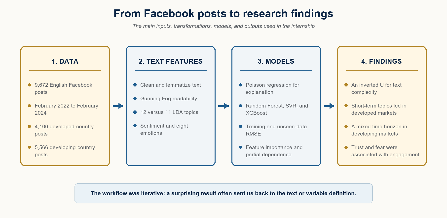
Parametric density models: a prominent class of methods assumes that the terminal risk-neutral distribution follows a particular parametric specification. One widely used approach models the distribution as a mixture of lognormal densities calibrated to observed option prices (Bahra, 1997; Melick and Thomas, 1997).

Parametric methods are computationally efficient and often yield economically interpretable measures of skewness, kurtosis, and tail risk. Their flexibility, however, is inherently constrained by the assumed functional form.

Dynamic option pricing models: rather than specifying the terminal distribution directly, structural approaches derive the implied density from an assumed stochastic process governing the evolution of the underlying asset price. Examples include stochastic volatility and jump-diffusion frameworks calibrated to observed option prices (Bates, 1995; Malz, 1995).

Within these models, the risk-neutral density emerges endogenously from the dynamics of the underlying asset under the risk-neutral measure. While theoretically appealing, such models are computationally intensive and sensitive to model misspecification.

Application

Implementing the Breeden and Litzenberger (1978) result in practice requires a continuum of European option prices written on the same underlying asset, all sharing a common maturity and spanning a continuous range of strike prices from zero to infinity. Under such idealized conditions, the risk-neutral density can be recovered directly from the cross-section of option prices (at a given maturity date).

In practice, however, listed option markets provide only a sparse and discrete grid of strike prices, typically concentrated around the at-the-money (ATM) region. The absence of a complete continuum of option strikes, particularly in the deep in-the-money and far out-of-the-money regions, necessitates the use of interpolation across observed strikes and extrapolation into the tails in order to recover a smooth and arbitrage-free implied risk-neutral distribution.

Required data

Constructing a risk-neutral distribution requires option chain data (a set of calls and/or puts) for a single maturity, along with the underlying asset price, the prevailing risk-free rate, dividend assumptions, at the exact observation time of the market data.

Such data can be obtained from both free and commercial data providers. One of the most accessible sources is Yahoo! Finance; however, freely available option data is often subject to inconsistencies such as wide bid–ask spreads, stale quotes, and incomplete cross-sectional coverage of strikes, all of which can materially distort empirical estimation of the risk-neutral distribution (RND).

For our application, we employ simulated option data to illustrate the derivation of the implied risk-neutral distribution from an option chain within a controlled and internally consistent setting. This ensures that the resulting distribution remains aligned with the theoretical framework developed above.

Extraction of the implied risk-neutral density

From the collected option chain data, we first apply a series of standard filtering procedures designed to remove illiquid and economically inconsistent observations. In empirical applications, this typically includes liquidity screens, moneyness and maturity filters, implied-volatility sanity checks, and no-arbitrage constraints to mitigate errors arising from stale quotes, asynchronous observations, and market microstructure noise. Since the dataset employed here is simulated and internally consistent by construction, these preprocessing steps can be largely omitted.

Figure 3 below presents the implied volatility smile obtained from the simulated European call option chain after numerical inversion of the Black–Scholes–Merton pricing model. The smile is interpolated using a natural cubic spline over a dense strike grid spanning the filtered strike range of 4,000 to 6,000, under the assumptions of an underlying spot price of $5,300, a continuously compounded risk-free interest rate of 5.2%, and a remaining time-to-maturity of 30 days. The resulting smooth volatility curve serves as the key intermediate input for constructing a continuous and differentiable call pricing function required for subsequent risk-neutral density extraction.

Figure 3. Implied Volatility Smile

Source: computation by the author (with python)

The interpolated implied volatility smile is subsequently utilized to reprice European call options across a finely discretized strike grid, thereby constructing a smooth numerical approximation of the cross-sectional call price surface. The option implied risk neutral density is then recovered by applying the Breeden Litzenberger operator, corresponding to the second partial derivative of discounted call prices with respect to strike, to the smoothed pricing function. Figure 4 illustrates the resulting risk neutral density extracted from the simulated European call option chain under an underlying spot level of $5,300, a continuously compounded risk-free interest rate of 5.2%, and a remaining time to maturity of 30 days.

Figure 4. Implied Risk-Neutral Distribution

Source: computation by the author (with python)

You can download the Python code provided below for generating simulated call option chain data and the option-implied risk-neutral distribution, as discussed above.

Alternatively, you can download the R code below with the same functionality as in the Python file.

Empirical issues

A primary limitation in empirical recovery of the risk-neutral distribution is the discrete nature of listed option strikes. The Breeden–Litzenberger framework assumes a continuum over strike space, whereas traded options are observed only on a sparse and uneven grid concentrated around the at-the-money region.

A second limitation arises from the unobservability of the distribution tails. Deep in-the-money and far out-of-the-money options are often illiquid or not quoted, implying that tail behaviour of the risk-neutral density must be inferred through extrapolation rather than direct market observation.

A separate issue is asynchronous option quotes. Since option prices across strikes are not necessarily recorded simultaneously, the resulting cross-section may embed timing mismatches, introducing bias in the reconstructed pricing function. This is typically addressed using end-of-day settlement data or synchronized snapshots.

In addition, different levels of market liquidity (due to different levels of bid ask spreads for example) across strikes introduces noise and heterogeneity in observed quotes. Illiquid contracts may exhibit stale or unreliable prices, which can distort the implied volatility surface even after basic filtering.

Finally, the reconstruction procedure does not explicitly impose no-arbitrage conditions or global smoothness constraints across strikes. As a result, when option prices are interpolated to form a continuous surface, the fitted call price function may exhibit local violations of convexity in strike space (e.g., small regions where butterfly spreads imply negative prices or non-monotonic curvature). Such violations are problematic because they imply the possibility of arbitrage and can lead to risk-neutral probability estimates that are not economically consistent.

Despite these limitations, the framework remains a useful reduced-form tool for extracting risk-neutral densities, provided appropriate smoothing and arbitrage constraints are imposed.

Real-life applications

Central Bank Monetary Policy Monitoring

Bahra (1997) and Kim (2009) suggest that policymakers extract ex-ante risk-neutral distributions (RNDs) from interest rate, equity, and currency options to assess market-implied expectations and uncertainty around policy decisions. Unlike futures prices, which only reflect the conditional mean, RNDs incorporate higher-order information such as skewness and kurtosis, allowing for a more complete assessment of perceived tail risks and macro-financial stress. For example, during the February 2007 equity sell-off, the European Central Bank (ECB, 2007) used option-implied probability distributions (“fan charts”) to assess whether the move reflected extreme tail risk and to track the evolution of market expectations after stabilization.

Value-at-Risk (VaR) Forecasting

Risk management units in investment banks use quantiles derived from implied RNDs to forecast extreme portfolio losses in a forward-looking manner. Compared to traditional historical simulation methods, RND-based approaches incorporate market-implied expectations and have been shown to provide improved performance relative to standard volatility-based models such as GARCH(1,1) (Chang, Chang, Huang, & Hsieh, 2011).

Systemic Risk and Stress Testing Indicator

Macroprudential regulators transform option-implied volatility surfaces into arbitrage-consistent risk-neutral distributions to quantify system-wide financial vulnerabilities. By aggregating tail-risk measures across equities, currencies, and interest rates, these distributions can be used to construct time-series indicators of systemic stress and cross-asset fragility (Malz, 2014).

Market Risk Aversion and Investor Sentiment Estimation

By combining option-implied risk-neutral distributions with empirical (physical) distributions, researchers can infer the market’s implicit risk preferences and aggregate degree of risk aversion (Bliss & Panigirtzoglou, 2004). This allows for the identification of time variation in investor sentiment and risk pricing across different investment horizons (Bliss & Panigirtzoglou, 2004; Gemmill & Saflekos, 2000).

Why should you be interested in this post?

The risk-neutral distribution is one of the few tools in finance that reveals how the market prices uncertainty based on the entire distribution of possible future states implied by option prices. It is widely used in practice to understand how the market is pricing downside risk, fat tails, and asymmetry that is directly used in volatility modelling, pricing, and risk management frameworks. From a practical perspective, it is one of the standard tools used to extract forward-looking information from option prices in both research and industry settings.

Useful resources

Academic research on option pricing

Black, F., & Scholes, M. (1973). The pricing of options and corporate liabilities. Journal of Political Economy, 81(3), 637-654.

Hull J.C. (2015) Options, Futures, and Other Derivatives, Eighth Edition, Global Edition, Chapter 14 – The Black-Scholes-Merton model, 299-320.

Merton, R.C. (1973). Theory of rational option pricing. The Bell Journal of Economics and Management Science, 4(1), 141-183.

Academic research on risk neutral distribution

Aït-Sahalia, Y., & Lo, A. W. (1998). Nonparametric estimation of state-price densities implicit in financial asset prices. The Journal of Finance, 53(2), 499-547.

Bahra, B. (1997). Implied risk-neutral probability density functions from option prices: Theory and application. Bank of England Working Paper Series, 66, 1-42.

Bates, D. S. (1991). The crash of ’87: Was it expected? The evidence from options markets. The Journal of Finance, 46(3), 1009-1044.

Bates, D. S. (1995). Testing option pricing models. NBER Working Paper Series, w5135, 1-53.

Bliss, R. R., & Panigirtzoglou, N. (2004). Option-implied risk aversion estimates. The Journal of Finance, 59(1), 407-446.

Breeden, D. T., & Litzenberger, R. H. (1978). Prices of state-contingent claims implicit in option prices. Journal of Business, 51(4), 621-651.

Chang, Y. C., Chang, C. L., Huang, H. T., & Hsieh, T. H. (2011). Value-at-Risk forecasting via option-implied risk-neutral density. Journal of Risk and Financial Management, 4(1), 56-83.

European Central Bank (ECB). (2007). Gauging stock market uncertainty using option-implied distributions. ECB Monthly Bulletin, April, Box 4, 31–32.

Figlewski, S. (2010). Estimating the implied risk neutral density for the U.S. market portfolio. In T. Bollerslev, J. R. Russell, & M. W. Watson (Eds.), Volatility and Time Series Econometrics: Essays in Honor of Robert F. Engle (pp. 43-69). Oxford University Press.

Gemmill, G., & Saflekos, A. (2000). How useful are market-implied probabilities for forecasting sharp changes in asset prices? An application to the UK general election. Market Expectations and the Implications for Monetary Policy, 203-223.

Kim, K. (2009). Monetary policy announcements and market expectations under different monetary policy regimes: An options-based approach. International Finance Discussion Papers (Federal Reserve Board), 977, 1-45.

Malz, A. M. (1996). Using option prices to estimate realignment probabilities in the European Monetary System: the case of sterling-mark. Journal of International Money and Finance, 15(5), 717-748.

Malz, A. M. (2014). A VaR-based systemic risk indicator. Federal Reserve Bank of New York Staff Reports, 668, 1-47.

Melick, W. R., & Thomas, C. P. (1997). Recovering an asset’s pdf from option prices: An application to crude oil during the Gulf crisis. Journal of Financial and Quantitative Analysis, 32(1), 91-115.

Neuhaus, H. (1995). The informational content of derivatives for monetary policy. Deutsche Bundesbank Discussion Paper Series 1: Economic Studies, 1995(03), 1-34.

Shimko, D. (1993). Bounds of probability. Risk, 6(4), 33-37.

Shreve, S. E. (2004). Stochastic calculus for finance II: Continuous-time models. Springer Science & Business Media.

About the author

The article was written in June 2026 by Saral BINDAL (Indian Institute of Technology Kharagpur, Metallurgical and Materials Engineering, 2024-2028 & Research assistant at ESSEC Business School).

▶ Discover all articles by Saral BINDAL

“Compound interest is the eighth wonder of the world. He who understands it, earns it … he who doesn’t, pays it.” – Albert Einstein

June 15, 2026May 28, 2026 by Hadrien PUCHE

Why do some financial portfolios grow at an explosive rate, while others seem to stagnate? The answer often lies in a mathematical phenomenon that Albert Einstein allegedly called the “eighth wonder of the world”: compound interest.

In this article, Hadrien PUCHE (ESSEC Business School, Grande École Program, Master in Management, 2023-2027) explores the mechanics of compound interest, to help you better understand how to include this concept to your own financial strategy or investments.

About Einstein and this quote

Albert Einstein

Albert Einstein is universally recognized as the father of modern physics, famous for the theory of relativity. While his primary focus was the universe, he possessed a deep appreciation for the beauty of mathematical patterns. Although the exact origin of this specific quote is a matter of historical debate, it perfectly captures the scientific essence of wealth creation: compounding is essentially the “physics” of capital.

To Einstein, compound interest was the ultimate proof that small, consistent actions can lead to massive, universal results over time.

Analysis of the quote

The core of Einstein’s idea is that understanding compound interest is a prerequisite for investing. If you view money linearly, you see a €1,000 investment as just a fixed sum, that can earn you a couple euros every month. If you view it through the lens of compounding, you see it as a seed, with a potential to grow into a couple thousand euros over many years.

This results in the following dichotomy in terms of financial literacy:

“He who understands it, earns it”: the investor who knows and understand compound interest reinvest his investment earnings, and create a self-sustaining loop where investments grow exponentially.
“He who doesn’t, pays it”: the individual who does not understand compound interest starts taking high-interest liabilities, such as credit card debt, and does not realize that he his the one paying for someone else’s exponential returns, as compound interest due on the debt create a bleeding process that can quickly lead to insolvency.

However, while Einstein’s quote presents compounding as a binary choice (either you understand it or not), modern financial economics introduces a vital optimization constraint: the Life-Cycle Hypothesis.

Early in your life, you may not have a lot of financial assets, but you do have a great “human capital” (your future earning potential).
As you age, your human capital converts into financial capital, as your future earning potential converts into actual earnings and financial capital.

As a result, you have to consider your total net worth as the sum of both types of capital :

Total wealth = human capital +financial capital

The key idea is that when you are young, you have a massive human capital that acts as a safety net, so you can afford to invest into high-risk high-reward assets, that will benedit the most from compounding. On the other hand, when you are older, following Einstein’s quote blindly would be a mistake : as you get closer to retirement, you should lower the risk of your financial capital, because you no longer have a human capital to replace it.

Samuelson (1969) and Merton (1969) proved mathematically that to maximize the compounding effect over time, an investor’s risk tolerance and portfolio composition must shift across the stages of life.

Ultimately, compound interest remains a neutral mathematical force; its structural impact on your life depends entirely on which side of the balance sheet you stand, and how dynamically you manage your assets across your life cycle.

My view on this quote

Einstein’s quote is a reminder that the greatest challenge in finance is not mathematics, but patience. We discussed the importance of patience in an article about the following quote from Warren Buffett: “The stock market is designed to transfer money from the impatient to the patient”. Read the full article here .

Most people fail to “earn” compound interest because they cannot endure the “boring” years, when the curve looks flat. However, if you respect the laws of physics that govern capital, you realize that you don’t need to be a genius to build wealth, you simply need to be disciplined enough to let the math do the work for you, and reach the exponential part of the curve.

Compound interest graph

This is exactly what any compound interest curve shows : you need to wait a long time until compound interest starts making a big difference with linear one.

The math behind compound interest

To move beyond the rhetoric, we must understand the formula that governs this “wonder.” Unlike simple interest, which is calculated only on the initial principal, compound interest is calculated on the principal plus the accumulated interest of previous periods.

The standard formula for the future value of an investment is:

FV formula

Where:

A = the future value of the investment
P = the principal investment amount
r = the annual interest rate (decimal)
n = the number of times that interest is compounded per unit t
t = the time the money is invested for

The most critical variable in this equation is t (time). Because it is an exponent, time has a disproportionate impact on the final result. This is why “time in the market” is vastly superior to “timing the market.”

The number of times interest is compounded per year, n, is also important because it reflects the speed of compounding. When interest is compounded more frequently (for example, daily rather than annually), each gain is reinvested sooner and can start generating additional returns within the same year. This accelerates the growth of the investment over time.

A technical case study about the cost of delaying your investments

We are now going to follow three different individuals, that are investing for their retirement (we do not consider public pensions). They adopt three distinct behaviors:

The first investor is well disciplined. He invests €200 every month throughout his 40 years long career.
The second investor wants to retire early. To do so, he invests €500 every month, but retires after only 20 years.
The third investor forgets about retirement until he his 55 years old. He wants to catch-up, so he invests €1000 every month, trying to catch-up with the other two, but he only has 10 years left until retirement.

How much money can each of these three investors expect to have for their retirement, and much will they be able to spend every month when retired? Download this Excel file and answer all three questions to find out.

Financial Modeling Exercise: To calculate the exact future values and monthly retirement allowances for each scenario, you can download the simulation model here: Excel Simtrade Compound Interest Exercise .

Analysis of the results

Table from the excel file

These simulations should prove to you the following points:

Spending more time in the markets is much more important than investing more: Investor C invested just as much as investor B, but because he did so in 10 years instead of 20, his final monthly pension is much lower. Similarly, despite contributing in total much less than the other two, investor A’s pension ends up being the largest one by far.
Catching-up when you are late is almost impossible: Q3 shows that investor C would have to invest €3,576 every month for 10 years to get the same pension as investor A. In real life, this would be very difficult to achieve without a high-paying job, whereas investor A only had to put aside €200 every month…

Ultimately, this exercise proves that the “cost of delay” is not linear, but exponential. Every year of procrastination at 25 years old costs much more than a year of procrastination at 55 years old.

Other resources

Merton, R. (1969), “Lifetime Portfolio Selection under Uncertainty: The Continuous-Time Case,” Review of Economics and Statistics, 51(3), pp. 247–257.
Samuelson, P. (1969), “Lifetime Portfolio Selection by Dynamic Programming,” Review of Economics and Statistics, 51(3), pp. 239–246.

About the Author

This article was written in May 2026 by Hadrien PUCHE (ESSEC Business School, Grande École Program, Master in Management, 2023-2027).

▶ Discover all articles by Hadrien PUCHE

“The philosophy of the rich and the poor is this: the rich invest their money and spend what is left. The poor spend their money and invest what is left.” – Robert Kiyosaki

June 15, 2026May 25, 2026 by Hadrien PUCHE

Is wealth a result of how much you earn, how much you spend, or how much you save? When it comes to personal finance, many assume that a higher salary is the only way to get rich. However, Robert Kiyosaki, the author of Rich Dad Poor Dad, suggests that the difference isn’t in the size of the paycheck, but in the size of the spending.

In this article, Hadrien PUCHE (ESSEC Business School, Grande École Program, Master in Management, 2023-2027) discusses Kiyosaki’s famous distinction between the “rich” and “poor” mindsets and analyzes the underlying financial mechanisms.

About Kiyosaki and this quote

Robert Kiyosaki is an American personal development author and businessman, who has become a well-known figure in financial education. He is famous for his 1997 book Rich Dad Poor Dad, which advocates financial independence through investing, real estate, and starting businesses.

Kiyosaki, Rich Dad Poor Dad Source : Amazon

This quote is deeply rooted in the first lesson of his book: “The rich don’t work for money.” Through the narrative of his “Rich Dad,” Kiyosaki explains that wealthy individuals prioritize their Asset Column, buying things that put money in their pockets, before addressing their Expense Column. By “investing first,” the rich ensure their wealth grows before lifestyle inflation takes hold.

Kiyosaki, Rich Dad Poor Dad Source : Singsaver

According to this framework, the distinctions are not just about the amount of money, but where it flows:

The Poor: their primary source of income is usually a job. This income flows directly into immediate expenses such as rent, food, and transportation. They typically possess no significant assets nor liabilities (because they can’t afford to buy any).
The Middle Class: like the poor, their primary source of income is a job. However, as their income rises, they often acquire what they perceive as assets but are actually liabilities (a house with a mortgage, a car with a loan, etc.). These liabilities create a cycle where a large portion of their income is diverted to debt payments before it even reaches their daily expenses.
The Rich: they focus on building their assets column first. Their income is primarily generated by assets such as real estate, stocks, bonds, and intellectual property. This passive income then flows into their income statement, covering their expenses and allowing for further investment back into more assets.

This visualization highlights why the “invest first” philosophy is so critical. While the middle class is often caught in a trap of working harder to pay for increasing liabilities, the rich use their income to buy things that eventually pay for their lifestyle.

It is important to note that Kiyosaki’s philosophy was heavily influenced by his mentor, the business philosopher Jim Rohn. Rohn frequently taught: “Poor people spend their money and save what’s left. Rich people save their money and spend what’s left.” Kiyosaki essentially refined this wording to emphasize “investing” over “saving,” reflecting a more aggressive approach to capital allocation.

The key difference between saving and investing is the willingness to take risks. Saving focuses on capital preservation, risk aversion and short-term liquidity, at the cost of a low yield, whereas investing means accepting risk (and / or illiquidity) in exchange for a greater return.

Analysis of the quote

The core idea behind the quote is a fundamental distinction between two different financial behaviors:

The ‘Rich’ behavior: invest first and then live off the rest. A rich person is someone who has reached a level of capital where they no longer have to care about the cost of daily living, so they can afford to invest the bulk of their income and spend the remaining without anxiety.
The ‘Poor’ behavior: live first, and then eventually invest what is left. A poor person must always address immediate survival needs first, leaving investing as a secondary (and often unreachable) goal.

However, if we look at the literal reality, the quote’s view on poor people’s behavior is quite unfair to them.

Statistics show that a significant portion of the population lives paycheck to paycheck (62% in the US according to PYMNTS, and 43% in France according to ADP), meaning they literally have nothing “left” after basic necessities. For them, the choice to “invest first” does not make sense at it is impossible for them to live properly and save.
Personal development gurus often argue that if you “think” like the rich, you will become rich. While a disciplined mindset is helpful, this quote can be seen as “unpractical” because it ignores the structural reality of low wages and the high cost of living.

Essentially, the quote is more about financial discipline than a literal description of social classes. It defines “rich” as someone who achieves freedom by making their money work for them, rather than being a slave to their expenses. It is a valuable financial lesson, even though the term ‘Poor’ would be better replaced by ‘Middle class’.

Financial concepts linked to this quote

Kiyosaki’s philosophy is a good opportunity for us to examine three key financial concepts that are linked to this quote: assets vs. liabilities, compound interest and the time value of money, and opportunity cost.

Assets vs. Liabilities

Kiyosaki’s most famous contribution is his simplified and cash-flow-centric way to define assets and liabilities. In traditional corporate accounting, an asset is broadly defined as an economic resource owned or controlled by an entity, whereas a liability is an obligation or debt owed to an external party. Under this conventional framework, a primary residence or a personal vehicle is classified as an asset because it possesses measurable intrinsic and market value.

However, Kiyosaki challenges this traditional view by narrowing the definitions down to a single variable: the direction of net cash flow.

An asset is strictly something that puts money in your pocket. This includes tangible and intangible holdings: rental properties, dividend-paying stocks, or a business that can run without your daily presence.
A liability is something that takes money out of your pocket. This often includes items that people mistakenly view as “investments”, such as a car or a primary residence. While these may have market value, they require constant outflows for monthly maintenance, insurance, and taxes without generating direct income, so Kiyosaki believes you should see them as liabilities.

This distinction is crucial, because many individuals mistakenly believe they are building wealth when they are actually accumulating liabilities, that require increasing amounts of cash flow to maintain. For a sophisticated investor, the goal is to use income to acquire assets that generate even more income, creating a self-sustaining loop.

This is the “Rich” mindset Kiyosaki is all about: you should target a life where the cashflows from your assets cover the expenses from your liabilities. This way, you no longer have to work for money, as your money is the one working for you.

Another benefit of assets is that they allow investors to multiply their returns through financial leverage. By borrowing other people’s money at a fixed borrowing rate of X%, and investing it in an income-generating asset for a return of Y%, as long as Y is greater than X, the investor captures a positive spread that maximizes their return on equity (ROE). Because Kiyosaki advises prioritizing the asset column, utilizing strategic debt becomes a primary mechanism to scale an investment portfolio far faster than organic cash savings would allow.

An important note on risk: Financial leverage is fundamentally a double-edged sword. While a positive spread ($Y > X$) exponentially accelerates wealth accumulation, leverage works both ways: it severely magnifies downside risk. If the asset’s returns fall or cash flows dry up while the mandatory debt service remains fixed ($Y < X$), the investor faces heavy financial stress, margin calls, or outright insolvency.

Compound Interest and the Time Value of Money

By “investing first,” an individual maximizes the time their money spends in the market. This is good because of one of the most important aspects of investing: compound interest.

Compounding interest is the process where the returns on an investment generate returns of their own the next year, creating an exponential growth curve over time.

Cover of Rich Dad Poor Dad by Robert Kiyosaki

As you can see on this graph, compound interest leads to exponential returns, whereas simple interest only leads to linear returns over time.

Compound interest works because of another key concept: the time value of money. The idea is that a dollar today is worth more than a dollar tomorrow because of its potential earning capacity (you could invest it and have more money tomorrow).

When a poor person waits to “invest what is left”, it also means missing more years of exponential growth for the capital, as the “cost” of waiting is not linear, but compounded.

Opportunity Cost

Every euro spent on a luxury item or an unnecessary expense carries an opportunity cost with it. In finance, capital is never free; every dollar tied up in a trade or a purchase is a dollar that isn’t earning a return for you. To truly calculate the price of a purchase, you must look beyond the sticker price and consider the “future value” that capital could have achieved if invested in a “risk-free” benchmark (or a diversified portfolio).

By spending first, you aren’t just losing the money today; you are losing the future wealth that money was destined to create.

As an example: If you spend €1,000 on a new phone today instead of investing it at a 7% annual return, the “real” cost of that phone over 10 years is actually ~$1,967. Over 30 years, that single €1,000 purchase represents an opportunity cost of over €7,600. This is why disciplined investors view market prices through the lens of intrinsic value rather than social status. By prioritizing spending, you are effectively selling your future financial freedom at a premium price for a temporary luxury.

The Life-Cycle framework and the rational borrowing phase theory

In Robert Kiyosaki’s popular framework, debt is viewed through a binary lens: it is either “good” (if it directly funds income-producing assets) or “bad” (if it is used for personal consumption). However, mainstream financial economics provides a more nuanced and structurally rigorous perspective through the lens of the Life-Cycle Hypothesis.

In the foundational models developed by Robert Merton and Paul Samuelson (1969), an individual’s total lifetime wealth is split into two distinct pillars:

Financial Capital: All tangible, investable assets in the traditional accounting sense.
Human Capital: The discounted present value of all future labor income.

What makes this framework highly compelling is how it redefines early-career balance sheets. At the start of a professional life, an individual’s financial capital is typically near zero, yet their human capital is at its absolute peak. From a corporate finance standpoint, this means young professionals are not asset-poor; rather, they possess a massive, illiquid asset that they ought to leverage through a strategic borrowing phase.

Total wealth as the sum of financial capital and human capital Source : ResearchGate

Taking on early liabilities (student debt, a first mortgage…) becomes economically rational when evaluated against the aggregate of both financial and human capital. In essence, this leverage is securely collateralized by expected future labor earnings.

Conversely, a rigid adherence to Kiyosaki’s precepts would discourage taking on debt that doesn’t immediately yield cash flow. In practice, this dogmatic view would mean avoiding early leverage entirely, disincentivizing investments in one’s own education and long-term human capital.

Why should you keep this quote in mind?

This principle serves as a vital warning against lifestyle inflation. As most people progress in their careers and earn more, they instinctively increase their spending: buying a bigger house, a faster car, or more expensive clothes.

By following the “poor” philosophy of spending first, their net worth remains stagnant regardless of their salary. Keeping this quote in mind forces you to prioritize your future self over current impulses.

My view on this quote

While the quote is mostly there to motivate people, I find it to be quite unpractical in its purest form. It presents a binary choice that does not consider the nuances of daily survival. You cannot simply “act rich” to become rich; the reality of personal finance is that you must first secure your basic needs before you can even begin to consider an investment strategy.

The practicality of this mantra heavily depends on the underlying national financial culture, like how people invest for their retirement.

In the United States, investing in equity markets is seen as a crucial mean of wealth building, particularly when pensions are mostly built through capitalization. Because of this, it makes sense to remind individuals that they need to invest first (including for their retirement) and spend after, because if they spend everything, they won’t be able to retire.
On the other hand, in countries like France, where most pensions are obtained through redistribution, people can afford to ‘forget’ to invest, as it won’t have devastating consequences on their retirement.

In my opinion, the wisest strategy is to target a middle ground. Rather than blindly investing every cent and hoping you have enough left for rent (a recipe for financial stress), one should start by making a rational budget. As an example, you can first take everything you really need to spend every month (rent, food, etc.) and then split the rest between leisure and savings. This way, you can manage your lifestyle within reasonable bounds.

Ultimately, simply copying the habits of the wealthy will never guarantee an entry into the 1%. However, by being careful about how you spend, you might not immediately become “rich” in the Kiyosaki sense, but you will certainly become less poor, and it will contribute to developing an analytic rigor that may be useful in other aspects of your personal or professional life.

Useful resources

Kiyosaki, R. T. (1997). Rich Dad Poor Dad. Warner Books.

Rich Dad Cash Flow Patterns and Wealth.

Merton, R. (1969). Lifetime Portfolio Selection under Uncertainty: The Continuous-Time Case. The Review of Economics and Statistics, 51(3), 247–257.

Samuelson, P. (1969). Lifetime Portfolio Selection by Dynamic Stochastic Programming. The Review of Economics and Statistics, 51(3), 239–246.

About the Author

This article was written in May 2026 by Hadrien PUCHE (ESSEC Business School, Grande École Program, Master in Management, 2023-2027).

▶ Discover all articles by Hadrien PUCHE

“October: this is one of the peculiarly dangerous months to speculate in stocks. The others are July, January, September, April, November, May, March, June, December, August and February.” – Marc Twain

June 15, 2026May 13, 2026 by Hadrien PUCHE

Is there ever a “safe” time to invest money in financial markets? Many investors spend their careers searching for the perfect seasonal window, waiting for “calmer” months to risk their capital, or fearing specific periods like the infamous “October effect”. However, Mark Twain, as a cynical observer of human nature, suggests that our search for a financial safe harbor in the calendar is completely pointless.

In this article, Hadrien PUCHE (ESSEC Business School, Grande École Program, Master in Management, 2023-2027) explores Twain’s satirical warning against market timing and why, for the undisciplined investor, every month is just as “peculiarly dangerous” as the others.

About Mark Twain and this quote

Mark Twain (the pen name of Samuel Clemens) was an American writer and humorist, but also a frequent (and often unsuccessful) speculator. Despite his literary success, Twain lost a lot of money on various financial bets (inventions and mining stocks), which likely fueled the irony found in his financial observations.

Marc Twain

Source: Wikipedia Commons

This specific quote originates from his novel Pudd’nhead Wilson (1894). The irony lies in its structure: he begins by singling out October as dangerous, tapping into the historical anxiety of market crashes, only to list every other month of the year as equally perilous. The message is clear: the market does not care about your calendar; it is a “psychological arena” where risk is constant.

Puddn’head Wilson

Analysis of the quote

Twain’s quote is a satirical commentary on market seasonality and the fundamental flaws of investor psychology. By breaking the quote into its two logical parts, we can better see how he dismantles the common myths of market timing.

“October: this is one of the peculiarly dangerous months to speculate in stocks.”

In this first half, Twain acknowledges the “October Effect” theory. While investors usually cite the crashes of 1907, 1929 and 1987 as evidence of this seasonal anomaly, Twain’s observation is particularly visionary as, remember, he wrote these words in 1894.

Yet, while collective fear and “animal spirits” can turn this into a self-fulfilling prophecy, there is little inherent mathematical reason why October is riskier than any other period.

“The others are July, January, September, April, November, May, March, June, December, August and February.”

This punchline targets two specific human tendencies:

The illusion of control: Investors often suffer from “historical bias,” searching for patterns where none exist. By labeling a specific month as “dangerous,” we falsely imply that the others must be “safe”.
The persistence of risk: Twain reminds us that market price movements (that can be moved by news or investors’ behavior) can exhaust your resources in April or August just as easily as in October. Financial bubbles and “manias” do not follow a calendar; they follow a cycle of displacement, euphoria, and eventually, panic.

Financial concepts linked to this quote

The three following financial concepts can help you better understand the quote and what it implies about finance: market timing vs. time in the market, the Efficient Market Hypothesis (EMH), and speculation vs. investment.

Market timing vs. time in the market

Speculators try to “time” the market by entering in “safe” months, and exiting before the “dangerous” ones. However, academic research suggests that trying to “time the market” is always suboptimal relative to spending more “time in the market”, and leads to worse returns (See Black Swans and Market Timing: How Not to Generate Alpha, Estrada, J. in the Journal of Investing).

The majority of long-term gains in stock markets occur on a small number of trading days each year, and missing just a few of those “best days” (which can happen in any month) can seriously reduce the total return.

daily returns repartition graph

Source: ReasearchGate

As you can see on this graph, most daily returns are near 0, whereas there only is a very small number of days with higher returns.

As the saying goes, “time in the market beats timing the market.” While concentration in time (timing) seeks a “free lunch,” diversification over time through long-term holding is a much more reliable path to wealth.

Check out this article to learn more about why time in the market beats timing in the market.

The Efficient Market Hypothesis (EMH)

The Efficient Market Hypothesis (EMH) suggests that markets are all rational, and instantaneously reflect all available information. If there were truly a “safe” or “dangerous” month, arbitrageurs would immediately exploit that information until the advantage disappeared. For example, if everyone knew October was dangerous and sold their stocks, prices would drop in September. Knowing that September is dangerous, they would sell the stocks in August, and prices would drop in August. Knowing that August in dangerous …

The point is that something that everybody knows about cannot be considered as an informational edge, because there is no way for you to make money over someone else who also know about it.

Overall, Twain’s quote challenges the idea that any predictable seasonal “free lunch” exists. Because the market is a “voting machine” driven by the aggregate expectations of all participants, any easily identifiable pattern is likely already priced into the current valuation.

Speculation vs. Investment

Twain specifically uses the word “speculate,” a term that in a financial context, is very different from “invest”.

Investment is based on disciplined fundamental analysis (examining earnings, balance sheets, management…) with the expectation of long-term value growth, regardless of short-term price volatility. An investor acts as a part-owner of a business, focusing on its intrinsic value rather than its daily market price.
Speculation, however, is essentially a bet on short-term price movement, often driven by market “noise,” rumors, or the “Greater Fool” theory. While an investment might be safe year-round if the underlying business quality is high, speculation is always “peculiarly dangerous” because it relies on “animal spirits” (the unpredictable human emotions and herd behavior that drive financial decisions).

The speculator is essentially a trader, trying to profit from the psychology of other participants, which makes him vulnerable to the “voting machine” nature of the short-term market. Unlike a long-term investor who can wait for a “valuation gap” to close, the speculator often faces the pressures of short selling costs, margin calls, or the lethal risk of a short squeeze. As Twain implies, this makes the speculator’s path dangerous in every month of the year, because they are not betting on the business itself, but on the timing of the crowd’s next move.

If you want something safer, all you have to do is investing instead of speculating. It will still be risky, as markets always are, but will be less risky.

Why you should always keep this quote in mind

You should see this quote as a necessary reality check against the urge to time the market. In finance, being “right” too early can lead to insolvency if the market’s irrationality outlasts your capital. This is famously discussed in the context of Keynes’s warning that markets can remain irrational longer than you can remain solvent.

Twain’s humor serves as a reminder that there is no “secret calendar” to success; the only true protection is discipline and a realistic assessment of risk.

My opinion on this quote

Twain’s core idea is absolutely right: in finance, the calendar is usually a distraction. Many retail investors wait for “the right time” to invest, only to watch from the sidelines as the market climbs over time. Statistically, studies on Dollar Cost Averaging (DCA) vs. Lump Sum Investing often show that investing immediately (Lump Sum) outperforms waiting for a dip, simply because markets tend to trend upward over time. However, DCA remains a powerful tool for the “psychological arena,” as it helps investors avoid the emotional cost of potentially entering the market at a peak.

Overall, the “danger” isn’t the month, but our own cognitive biases. Many buy when there is “euphoria” and sell when there is “panic,” regardless of whether it’s June or December. Instead of watching the calendar, we should focus on the quality of our assets and our ability to remain solvent through the inevitable periods of market irrationality.

However, I disagree with Marc Twain use of the word ‘speculate’. If your goal is to speculate and not investing, then the best months of the years should be the most dangerous ones, as they allow for more market movements and more quick profit opportunities. In that sense, for a speculator, Twain’s insights would be that October is not more profitable than the others months to speculate, not exactly what Twain intended to say, but it does show how Twain was wrong to try to speculate instead of simply investing is money in the market without thinking too much about it.

Useful resources

Books

Twain, M. (1894). Pudd’nhead Wilson.

Malkiel, B. G. (1973). A Random Walk Down Wall Street.

Shiller, R. J. (2000). Irrational Exuberance.

Academic Research

Shleifer, A., & Vishny, R. W. (1997). The Limits of Arbitrage. The Journal of Finance, 52(1), 35-55. Available via JSTOR. (Explains why markets can stay irrational longer than an arbitrageur can remain solvent ).

Estrada, J. (2008). Black Swans and Market Timing: How Not to Generate Alpha. The Journal of Investing, 17(3), 20-34. Available via IESE Business School. (Demonstrates how missing just a few of the market’s best days can drastically reduce long-term returns).

Sharpe, W. F. (1991). The Arithmetic of Active Management, Financial Analysts Journal, 47(1), 7-9. Available via Stanford University. (Details why the average market participant must achieve the market return before fees ).

About the Author

This article was written in May 2026 by Hadrien PUCHE (ESSEC Business School, Grande École Program, Master in Management, 2023-2027).

▶ Discover all articles by Hadrien PUCHE

May 2026 – Bond Markets: Key Articles from the SimTrade Blog

May 2, 2026 by Prof. François LONGIN

Most Read Articles about Bonds on the SimTrade Blog

This monthly selection highlights key articles on bond markets, chosen based on their pedagogical value, practical relevance, and readership engagement. Bond markets have been selected as a central theme due to their critical role in the transmission of monetary policy, the formation of interest rates, and the valuation of financial assets in the current macro-financial environment. They are also particularly relevant in a context of heightened geopolitical uncertainty, which may influence yield dynamics through its impact on inflation expectations, energy prices, and global risk premia. In both the United States and the euro area, government bond yields have increased by around 20 to 30 basis points in recent weeks (depending on maturities) reflecting upward revisions in inflation expectations and a repricing of monetary policy trajectories.

Financial techniques

▶ Georges WAUBERT Bond valuation

▶ Alexandre LANGEVIN Duration and Convexity: Measuring Bond Price Sensitivity to Interest Rates

▶ Georges WAUBERT Bond risks

Types of bonds

▶ Nithisha CHALLA US Treasury Bonds

▶ Akshit GUPTA Green bonds

▶ Anant JAIN Social Impact Bonds

▶ Akshit GUPTA Eurobonds

Profesional experiences

▶ Tianyi WANG My internship experience as an analyst assistant at China Bond Rating

▶ Andrea ALOSCARI My Internship Experience in the Corporate & Investment Banking division of IMI – Intesa Sanpaolo

▶ Chloé ANIFRANI My experience as an Asset Management Sales Assistant for Amplegest

A solid understanding of bond markets is essential for interpreting interest rate dynamics, assessing monetary policy transmission, and making informed investment decisions, which makes these articles particularly valuable for students and aspiring finance professionals.

The Rise of Algorithmic Trading: From Simple Strategies to Machine Learning

April 30, 2026 by Anis MAAZ

In this article, Anis MAAZ (ESSEC Business School, Global Bachelor in Business Administration (GBBA), 2023-2027) explains how algorithmic trading works, from rule-based strategies like market making, arbitrage, and momentum to modern machine learning models and the systems that run them. The goal of this post is to give a clear, realistic overview of today’s algo landscape, its methods, data and infrastructure needs, and the risks and controls traders must understand before building or adopting an automated strategy.

What “algorithmic trading” means

Algorithmic trading is the use of computer programs to make and execute trading decisions according to predefined rules. These rules can be simple, such as splitting a large order into smaller pieces to reduce market impact, or more sophisticated, such as detecting short term patterns in prices, volumes, or order book dynamics. The goal is not necessarily to trade fast, but to trade systematically and consistently, removing emotion and human latency from the process.

Algorithmic trading now dominates global markets. According to JP Morgan and Bloomberg estimates, it accounts for roughly 60–73% of U.S. equity trading volume, 40–50% in European equities, around 80% in FX spot markets (BIS Triennial Survey, 2022), and over 70% in futures markets. The evolution has been dramatic: less than 15% of U.S. equity volume in the early 2000s, past 50% by 2008, and a peak above 70% during 2009–2012 with the rise of high-frequency trading. It has since stabilized between 60% and 75% as regulation tightened and the industry consolidated around a few dominant players.

Why it grew so fast?

Three forces drove adoption. First, markets became electronic and faster, so speed and precision started to matter in everyday execution. Second, data and computing became cheap: brokers and exchanges exposed APIs, cloud resources got affordable, and open-source libraries appeared. Third, microstructure itself changed: most trading now occurs on limit order books where tiny, frequent price changes reward consistency and careful cost control. Together, these factors made rules based automation both feasible and attractive for firms and independent traders.

The ecosystem is driven by several types of players: high-frequency trading firms (Citadel Securities, Virtu Financial, Jump Trading, Jane Street) that dominate market making and short-term arbitrage; quantitative hedge funds (Renaissance Technologies, Two Sigma, D.E. Shaw) that run systematic strategies on longer horizons; investment banks (Goldman Sachs, JP Morgan) operating algorithmic execution desks for clients; asset managers (BlackRock, Vanguard) using algorithms for portfolio rebalancing; and a fast-growing retail segment leveraging platforms like Interactive Brokers, Alpaca, or MetaTrader.

How a typical algorithmic setup works (without jargon)

Under the hood, most systems share four components. A signal suggests “buy,” “sell,” or “do nothing,” based on patterns the designer expects to repeat. Risk controls limit position size, daily losses, and exposure across instruments, and can stop the system if limits are hit. An execution module decides how to place orders, market or limit, how aggressively to join or improve the queue, and how to behave in volatile moments. Finally, a testing loop checks ideas on past data (backtests), then in small live trials (forward tests), and monitors production to catch problems or errors early. This last step is the most important one to verify the algorithm really works before committing significant capital.

Machine learning, when used, lives mainly in the signal step: models learn patterns from large datasets such as order book features or news sentiment. It can improve accuracy, but it also adds failure modes such as overfitting (the model memorizes the past instead of learning real patterns) and model drift (the market changes and the model becomes obsolete), so governance and validation become central. Academic research highlights both sides of this automation: Hendershott, Jones, and Menkveld (2011) show that algorithmic trading improves liquidity and makes quotes more informative; Brogaard, Hendershott, and Riordan (2014) find that high-frequency traders contribute to price discovery; but Kirilenko et al. (2017), studying the 2010 Flash Crash, demonstrate how automated systems can amplify volatility during stress episodes.

What algorithms actually do: strategy families in practice

Market making is like being a middleman who constantly buys and sells throughout the day, making money from the small difference between buy and sell prices (the “spread”), while keeping inventory balanced and adjusting prices or stepping back when the market gets too volatile. Firms like Citadel Securities and Virtu Financial dominate this activity on U.S. equities.
Arbitrage is when you spot the same (or very similar) asset trading at different prices in different places, like a stock and its future, or two related ETFs, and you quickly buy the cheaper one while selling the expensive one to lock in a small, low-risk profit. During big crashes or market events, arbitrage opportunities can be captured by algorithms in milliseconds. For example, in October 2025 when Trump announced China tariffs, the crypto market crashed and USDe was priced at $0.65 on one platform for a few seconds while still trading at $1 on another.
Momentum and mean reversion are two simple trading approaches: momentum bets that a price move will continue in the same direction, while mean reversion bets that extreme moves will bounce back toward normal. Alongside these, execution algorithms (such as VWAP or TWAP) do not predict anything but help traders buy or sell large orders quietly and cheaply by blending into the market’s natural flow.

A simple numeric example

Imagine you are running a small trading bot that makes €0.01 profit every time it buys and sells a share. If it does this 1,000 times in a day, you would expect €10 in profit. But after paying fees to the exchange, your broker, and losing a bit of money on timing (called “slippage”), you are actually left with only €2. Here’s the problem: if the market gets a little more chaotic and your timing losses increase by just €0.004 per share, that €2 profit completely disappears and you start losing money. This is why successful trading firms are obsessed with speed, positioning in the order queue, and keeping costs as low as possible: when you are making thousands of tiny trades, even the smallest extra cost can wipe out all your profits. This is also why trading firms increasingly recruit technical profiles (developers, data engineers, quants) to build and maintain these algorithms.

Typical risks and how professionals address them

Model error and overfitting: a backtest can look perfect by accident. Good practice includes out-of-sample tests, stress scenarios, and small-size live trials before scaling up.
Execution and infrastructure: partial fills, slippage, network outages, or API changes can break assumptions. Firms use pre-trade checks, kill switches, redundancy, and post-trade analytics to limit damage.
Regime shifts and liquidity: relationships that held in calm markets can fail in stress. Circuit breakers, dynamic limits, and stricter quoting rules help, but strategy design must assume bad days will come, as shown by the 2010 Flash Crash where the Dow Jones lost nearly 1,000 points in minutes.
Market manipulation and regulation: practices like spoofing (placing fake orders to mislead other participants) or layering are banned under MiFID II in Europe and Dodd-Frank in the U.S. Regulators (ESMA, AMF, SEC, FCA) actively monitor algorithmic activity. In 2020, JP Morgan paid a record $920 million fine for spoofing in precious metals and Treasury markets, showing that even the largest institutions are held accountable.

Machine learning: value and limits

Machine learning can find trading patterns in huge amounts of data: price movements, order flows, news headlines, but more complicated does not always mean better. In practice, many teams prefer simpler models they can actually understand and explain over fancy “black box” systems. What really matters is control: who approves the model, how you track changes, what you do when it stops working, and how to shut it down safely. Regulators have made it clear that even if you are using AI, you are still responsible for what it does, MiFID II explicitly requires firms to test, document, and supervise their algorithms.

What this means for traders and firms

For big institutions, algorithms are now standard tools: they provide liquidity, route orders, and track costs in real time. For individual traders, algorithms offer discipline and consistency, but they also expose weaknesses fast: if your costs are too high or your strategy is fragile, automation will show you, sometimes the hard way, for example by losing all the capital you allocated to the algorithm. The real edge is not just having a clever formula; it is combining a small but reliable signal with strict risk rules, careful execution, and constant monitoring.

Conclusion

Algorithmic trading went from rare to normal because it matches how modern markets work: fast, electronic, and data-heavy. The strengths are speed, scale, and consistent rule-following; the weaknesses show up when controls break, data gets messy, or market conditions suddenly change. The best approach is a hybrid: humans set the rules and limits, machines execute consistently and report back. When this works, small repeatable advantages add up over time. When it doesn’t, automation just makes mistakes happen faster and at a higher scale, which is exactly why regulation and human oversight remain essential.

Why should I be interested in this post?

Algorithmic trading sits at the intersection of markets, data, and technology, now core to execution and price formation globally. Understanding rule-based and ML-driven strategies builds skills in market microstructure, data analysis, and risk control. For business and finance students, these are foundational for roles in trading, quant research, fintech, and portfolio management.

Useful Resources

Federal Reserve (2020) (IFDP) — Rise of the Machines: Algorithmic Trading in the Foreign Exchange Market (Full Paper Updated in 2020)

CSEF (2024) The Rise of Algorithmic Trading: Implications for Price Elasticity and Market Competitiveness

Equiti (2024) What is Algorithmic trading?

Hendershott, T., Jones, C. M., & Menkveld, A. J. (2011). Does Algorithmic Trading Improve Liquidity?

When Machines Beat Bias: What Algorithmic Trading Teaches Us About Rationality

About the author

The article was written in April 2026 by Anis MAAZ (ESSEC Business School, Global Bachelor in Business Administration (GBBA) 2027).

▶ Discover all articles by Anis MAAZ

Why Retail Option Strategies Underperform: Payoffs, Probabilities, and the Cost of Speculation

April 18, 2026 by Alexandre LANGEVIN

In this article, Alexandre LANGEVIN (ESSEC Business School, Global Bachelor in Business Administration (BBA), 2022-2026) examines why retail option strategies frequently underperform — that is, generate returns below a passive buy-and-hold benchmark or lose money outright — despite offering payoff profiles that appear attractive on paper. The article explains the structural mechanics behind four common strategies, identifies the sources of systematic drag, and illustrates how the gap between theoretical upside and realized performance emerges even before behavioral factors are considered.

Introduction

Options are among the most versatile yet complex instruments in financial markets. They can hedge risk, generate income, or express a directional view with defined downside (Hull, 2012). Yet a growing body of evidence suggests that retail investors who trade options systematically underperform both the market and their own expectations (Barber and Odean, 2000; de Silva, So and Smith, 2024). The question is not whether options are useful tools; they plainly are. The question is whether the specific strategies retail investors tend to favor are structurally suited to delivering the outcomes they expect.

The answer, in most cases, is that they are not. The gap between the payoff diagram and realized performance is not primarily attributable to adverse price realizations. It is embedded in the mechanics of how options are priced, how time erodes their value, and how the probability of profit is systematically lower than the shape of the payoff curve implies. Understanding these mechanics is the first step toward using options more deliberately.

How an Option Payoff Works

An option gives its buyer the right, but not the obligation, to buy (call) or sell (put) an underlying asset at a fixed price — the strike — on or before expiry. The buyer pays a premium for this right. At expiry, the profit or loss is determined entirely by the final price of the underlying relative to the strike.

For a long call: the option expires worthless if the underlying finishes below the strike. Above the strike, the buyer receives the difference between the final price and the strike. The buyer pays the premium upfront when entering the position; profit or loss at expiry therefore equals the intrinsic value minus this initial cost. The breakeven is therefore the strike plus the premium. For a long put, the logic is symmetric: the option has value if the underlying falls below the strike, and the breakeven is the strike minus the premium. Throughout this article, net profit or loss refers to the outcome at expiry after accounting for the premium paid upfront. The net profit or loss formula for a long call is:

Long call payoff formula

These payoff diagrams look appealing. The downside is capped at the premium paid; the upside is theoretically unlimited for calls and capped at the strike price minus the premium paid for puts (since the underlying cannot fall below zero) for puts. What the diagram does not show is the probability attached to each outcome.

The Four Strategies: Structure and Mechanics

The Excel model accompanying this article covers four strategies commonly used by retail investors. Each illustrates a distinct structural trade-off.

The following four strategies represent the most common approaches used by retail option traders, ranging from directional speculation to income generation.

Long Out-of-the-Money (OTM) Call. An option is out-of-the-money when exercising it immediately would produce no value — the strike is above the current price for a call, or below it for a put. In the illustrative example, SPY trades at $540. A call with a $560 strike costs $5.20. Breakeven is $565.20, requiring a 4.7% move in the underlying just to recover the premium. Below $560 at expiry, the entire $5.20 is lost. Above $565.20, the trade turns profitable. The net profit or loss is positively skewed and theoretically unlimited, which explains its appeal. The structural problem is that an OTM call requires the underlying to move by more than the market already expects, because the premium reflects that expected move.

A worked example illustrates the arithmetic. Suppose SPY closes at $575 at expiry. The intrinsic value of the $560 call is $575 − $560 = $15. Net profit per share = $15 − $5.20 = $9.80, or $980 per contract (one contract = 100 shares) — a return of 188% on the premium paid. Now suppose SPY closes at $550 instead. The call expires worthless; the loss is the full premium of $5.20 per share, or −$520 per contract. These two outcomes — $980 profit vs. −$520 loss — illustrate the asymmetry. The upside is real, but the full loss scenario is far more probable: SPY must rise more than 4.7% simply to break even, and more than that to generate meaningful profit.

Long OTM Put. A $520 put on SPY trading at $540 costs $4.80. Breakeven is $515.20, requiring a 4.6% decline. Like the OTM call, the put must overcome both the out-of-the-money gap and the premium cost before generating any return. In calm markets, the probability of hitting breakeven by expiry is well below what the payoff diagram implies.

Bull Call Spread. Buying the $550 call and selling the $570 call reduces the net cost to $5.30 (long premium $8.50 minus short premium $3.20). Breakeven falls to $555.30, and maximum profit is capped at $14.70 per share if SPY finishes above $570. The spread trades unlimited upside for a lower entry cost and a higher probability of profit compared to the naked call. The payoff formula is:

Bull call spread payoff formula

It is a more disciplined structure, but it still requires a meaningful directional move, and the profit ceiling is fixed regardless of how far the underlying moves above the upper strike.

Covered Call. An investor who holds 100 shares purchased at $540 sells a $560 call for $5.20. Breakeven falls from $540 to $534.80. If SPY finishes below $560, the investor keeps the premium and the position. If SPY finishes above $560, the shares are called away and the investor captures only $25.20 per share in total profit, regardless of how far the stock has risen. The strategy generates income but structurally caps the upside.

Figure 1. Payoff diagrams at expiry for the four strategies (illustrative inputs).
Option payoff diagrams
Source: computation by the author.

The Structural Sources of Underperformance

Three structural factors — theta decay, the volatility risk premium, and breakeven mechanics — explain why retail option strategies systematically underperform, independently of any behavioral bias.

Theta decay. Options lose value over time as expiry approaches. This decay is not linear; it accelerates sharply in the final weeks before expiry. A 30-day option that has lost 30% of its value in the first two weeks may lose the remaining 70% in the last two. Retail investors who buy short-dated options and hold them without a clear exit plan are running against the clock. The underlying must move quickly and decisively; a slow drift in the right direction is often not enough to overcome the daily erosion in time value. De Silva, So and Smith (2024) document that retail investors systematically purchase options ahead of anticipated volatility spikes, only to suffer double-digit percentage losses as volatility collapses and time value erodes post-announcement.

The volatility risk premium. Implied volatility — the level of volatility priced into an option’s premium — is persistently higher than realized volatility on average. This gap is the volatility risk premium, and it represents a systematic transfer of wealth from option buyers to option sellers. When you buy an option, you are paying for a level of volatility that, on average, does not materialize. Market makers and institutional sellers collect this premium consistently over time; retail buyers pay it. Broadie, Chernov and Johannes (2009) show that the apparently large returns to put-selling strategies are fully explained by compensation for bearing this volatility risk — what looks like alpha is largely a risk premium that option buyers are systematically on the wrong side of.

Breakeven mechanics. The breakeven calculation makes the structural difficulty explicit. For a long OTM call with a 4.7% breakeven requirement, the underlying must rise by 4.7% before expiry simply to recover costs. Historically, the probability of a large-cap equity index moving 5% or more in a given month is well below 50%. The payoff diagram shows what happens if the move occurs; it does not show how often it does. Most retail option buyers look at the profit region of the diagram without adequately pricing in the probability of reaching it. Barber and Odean (2000) document a closely related pattern in equity trading: retail investors systematically overestimate their ability to generate above-market returns, a bias that is amplified in options markets by the apparent leverage and lottery-like payoffs.

Transaction costs and taxes. A fourth source of drag, often overlooked, is the cost of trading itself. Retail investors typically pay per-contract commissions, and bid-ask spreads on options are wide relative to the premium — particularly for short-dated or illiquid contracts. On a $5.20 premium, a $0.10 spread represents nearly 2% of the position cost before any price move occurs. Capital gains taxes on short-term option profits further reduce net returns. These costs do not appear on payoff diagrams but compound the structural disadvantages described above.

Excel Model

The Excel model below contains four sheets — Long OTM Call, Long OTM Put, Bull Call Spread, and Covered Call — each following the same structure: an input table with yellow input cells, a payoff table across a range of expiry prices, and a payoff diagram with a breakeven marker. All inputs are illustrative and can be modified freely. The payoff columns and chart update automatically when inputs change.

Figure 2. Bull Call Spread sheet: inputs table and payoff formula.
Bull Call Spread inputs table
Source: computation by the author.

Why should I be interested in this post?

Options appear in equity research, derivatives desk interviews, and structured product discussions at banks and asset managers. Beyond the professional context, understanding why certain strategies structurally underperform is relevant for anyone who trades independently or advises clients on portfolio construction. The payoff diagram is the beginning of the analysis, not the end. Knowing how to read the probability distribution behind it is what separates informed use from speculation.

Useful resources

Academic research

Barber, B.M. and Odean, T. (2000) Trading Is Hazardous to Your Wealth: The Common Stock Investment Performance of Individual Investors, Journal of Finance, 55(2), 773-806. Available at https://faculty.haas.berkeley.edu/odean/papers%20current%20versions/individual_investor_performance_final.pdf

de Silva, T., So, E.C. and Smith, K. (2024) Losing is Optional: Retail Option Trading and Expected Announcement Volatility, Review of Finance, 30(2), 489-535. Available at https://www.timdesilva.me/files/papers/losing_optional.pdf

Broadie, M., Chernov, M. and Johannes, M. (2009) Understanding Index Option Returns, Review of Financial Studies, 22(11), 4493-4529. Available at https://business.columbia.edu/sites/default/files-efs/pubfiles/3964/broadie_chernov_johannes.pdf

Hull, J.C. (2012) Options, Futures, and Other Derivatives, 8th edition, Pearson.

About the author

This post was written in April 2026 by Alexandre LANGEVIN (ESSEC Business School, Global Bachelor in Business Administration (BBA), 2022-2026). Alexandre is interested in derivatives markets, options trading, and quantitative approaches to portfolio analysis.

▶ Discover all articles by Alexandre LANGEVIN.

The Shiller P/E (CAPE) Ratio: Measuring Long-Run Market Valuation

April 18, 2026April 17, 2026 by Alexandre LANGEVIN

In this article, Alexandre LANGEVIN (ESSEC Business School, Global Bachelor in Business Administration (BBA), 2022-2026) explains the Shiller P/E ratio, also known as the CAPE ratio: a valuation tool that adjusts for the business cycle to give a more reliable picture of whether equity markets are cheap or expensive.

Introduction

Every investor knows the price-to-earnings (P/E) ratio: divide the current market price by earnings per share and you get a simple measure of how much the market is paying for each dollar of profit. It is one of the most widely quoted metrics in equity analysis. But it has a structural flaw: earnings are cyclical. In a recession, they collapse, making the P/E look artificially inflated even when prices have barely moved. In a boom, they surge, making markets appear cheap when they may not be. A single year of earnings is a poor basis for a long-term valuation judgment.

Robert Shiller, a Yale professor and 2013 Nobel laureate in economics, proposed a simple fix. His ratio replaces one year of earnings with the average of the past ten years, adjusted for inflation. The result is a smoother, more stable measure of valuation that filters out the noise of the business cycle and allows for meaningful comparisons across time.

The Problem with Standard P/E

Consider the S&P 500 in 2009, shortly after the financial crisis. Prices had fallen sharply, but earnings had fallen even further, with many companies reporting losses. Standard P/E spiked above 100 at certain points, not because markets were expensive, but because the denominator had collapsed. An investor reading that number at face value might have concluded the market was dangerously overvalued, when it was near a generational buying opportunity.

The opposite problem occurs at cycle peaks. Strong earnings in boom years compress P/E ratios, making markets look reasonable just before a downturn. Standard P/E captures both price and the cyclical position of earnings simultaneously, making it hard to separate valuation from timing.

The CAPE Ratio: Construction and Formula

Shiller’s solution is to replace single-year earnings with the average of real earnings over the previous ten years. A ten-year window spans a full business cycle, smoothing out both recessions and booms. The formula is:

CAPE ratio formula

where P is the current market price, E_t are reported earnings in year t, CPI₀ is the current price index, and CPI_t is the price index in year t. The inflation adjustment ensures that past earnings are expressed in today’s dollars, making them directly comparable to recent figures.

In the Excel model, each annual earnings figure is the average of the 12 monthly observations in Shiller’s dataset. Shiller himself constructs monthly earnings by interpolating S&P four-quarter totals, so the monthly series is a smooth continuous estimate rather than actual reported monthly results. The current S&P 500 price used is the April 9, 2026 closing price of $6,824.66, sourced from Yahoo Finance. The CPI reference is the February 2026 release from the U.S. Bureau of Labor Statistics.

Historical Record and Market Signals

Shiller’s dataset goes back to 1871, giving the ratio an exceptionally long historical record. The average CAPE over that full period is approximately 17.7 and the median around 16.6. These serve as rough benchmarks: readings significantly above the average suggest the market is expensive relative to long-run earnings capacity, while readings well below suggest the opposite.

The ratio’s most cited applications came before two of the largest crashes of the modern era. In December 1999, at the peak of the dot-com bubble, the S&P 500 CAPE reached 44.2, more than double its historical average. Shiller published Irrational Exuberance that same year, arguing on the basis of CAPE that US equities were severely overvalued. The S&P 500 subsequently fell by nearly 50% over the following two years. In August 2007, CAPE rose above 26 before the financial crisis and another major decline.

At the other extreme, CAPE dropped to around 8.5 in August 1982, one of its lowest post-war readings, preceding one of the strongest bull markets in US history. As of April 9, 2026, our model gives a CAPE of approximately 38.8, well above the historical average.

Figure 1. CAPE ratio at key historical market turning points (S&P 500, selected monthly readings). Source: Robert J. Shiller, econ.yale.edu; computation by the author.
CAPE historical chart
Source: computation by the author.

Excel Model

The Excel model below computes the CAPE ratio from Shiller’s raw data. It contains four sheets: a source data sheet copied directly from Shiller’s dataset, a CAPE Calculator that pulls ten-year annual averages and applies the inflation adjustment, a Historical Context sheet with key turning points, and a Read Me. The starting year of the ten-year window is adjustable, and the model updates automatically when price or CPI inputs are changed.

Figure 2. CAPE Calculator: ten-year window of inflation-adjusted earnings and resulting CAPE ratio.
CAPE calculator Excel screenshot
Source: computation by the author.

Interpretation and Limitations

What CAPE tells you. Shiller’s own research found a strong negative relationship between starting CAPE and subsequent 10-year real returns for the S&P 500: high CAPE tends to precede lower decade-long returns, and low CAPE tends to precede higher ones. The relationship is not mechanical and does not predict timing, but it is one of the more robust long-run return predictors in the academic literature.

The interest rate objection. The most common criticism is that CAPE ignores the level of interest rates. When rates are structurally low, investors rationally accept higher valuations because the alternatives offer little return. Some analysts argue that elevated CAPE readings since 2010 partly reflect lower rates rather than pure overvaluation. This debate is unresolved.

Accounting changes. Reporting standards for earnings have evolved significantly since the 1870s, particularly around goodwill and write-offs. Some researchers argue that modern reported earnings are not strictly comparable to historical figures, making century-long CAPE comparisons imperfect.

Not a timing tool. Investors who sold equities in 1996 because CAPE was already above its long-run average missed four more years of exceptional gains before the dot-com peak. CAPE is a signal about long-run expected returns, not a predictor of short-term price moves.

Why should I be interested in this post?

Valuation metrics appear in equity research, asset allocation decisions at investment managers, and macro discussions at private banks. The CAPE ratio is referenced in strategy notes, central bank research, and academic papers on return predictability. Understanding what it measures, how it is built, and what its limits are is practical knowledge for anyone working in equities or asset management — and one of the cleaner examples of how academic research translates directly into a practitioner tool.

Useful resources

Academic research

Campbell, J.Y. and Shiller, R.J. (1988) Stock Prices, Earnings, and Expected Dividends, Journal of Finance, 43(3), 661-676. Available at scholar.harvard.edu.

Bunn, O. and Shiller, R.J. (2014) Changing Times, Changing Values: A Historical Analysis of Sectors within the US Stock Market 1872-2013, NBER Working Paper No. 20370. Available at nber.org.

Data sources

Shiller, R.J. Online Data, Yale University. S&P 500 price, earnings, CPI, and CAPE data from 1871 to present.

S&P 500 current price: Yahoo Finance.

CPI reference: U.S. Bureau of Labor Statistics, Consumer Price Index release.

SimTrade

SimTrade Courses

About the author

The article was written in April 2026 by Alexandre LANGEVIN (ESSEC Business School, Global Bachelor in Business Administration (BBA), 2022-2026).

▶ Discover all articles by Alexandre LANGEVIN.

About Petrini Valores

Trading in practice: what the desk actually looks like

Agency, intermediation, and principal trading: three different jobs

Pricing illiquid bonds: when there is no obvious answer

Primary market underwriting: when commitment meets reality

FX mismatches and capital controls: the Argentine laboratory

When models break: the lesson of negative oil prices

The most important rule on a trading desk

Argentina: the best trading school you never attended

Financial concepts related to this article

Principal trading and inventory risk

Underwriting syndicate and book runner

Dutch auction in primary bond markets

Blue-chip swap rate and capital controls

Why should I be interested in this post?

Related posts on the SimTrade blog

Useful resources

Academic research

Business resources

About the author

Understanding the challenge of options trading

What exactly is delta?

The principle of delta neutrality

The dynamic nature of delta

Hedging a single option versus a book of options

Re-hedging and trading costs

Why delta hedging matters

Securing the bank’s margin

A practical example

Common misconceptions

Conclusion

Why should I be interested in this post?

Related posts on the SimTrade blog

Useful resources

About the author

About the company

My internship

My missions

Required skills and knowledge

What I learned

Financial concepts related to my internship

Cost and Budget Management

Change Management

Due Diligence

Why should I be interested in this post?

Related posts on the SimTrade blog

Useful resources

About the author

From private banking to markets

About the company

My apprenticeship

Life on the trading floor

What I learned

Financial concepts related to my professional experience at HSBC

Market Liquidity

Collusion Risk

Profit and Loss (P&L)

Why should I be interested in this post?

Related posts on the SimTrade blog

Useful resources

About the author

Introduction

About Koragence

My experience as founder and President

My main responsibilities

Required skills and knowledge

What I have learned

The invisible cost of a fragmented information system

Integration has become a central management issue

Artificial intelligence changes the economics of software and automation

Economic, financial and business concepts related to my founder experience

Transaction costs and the make-or-buy decision

Return on investment and payback period

Operating leverage and reusable assets

Why should I be interested in this post?

Related posts on the SimTrade blog

Useful resources

Academic research

Business resources

About the author

Determining K₀