Implied Volatility and Option Prices

December 23, 2025December 23, 2025 by Saral BINDAL

In this article, Saral BINDAL (Indian Institute of Technology Kharagpur, Metallurgical and Materials Engineering, 2024-2028 & Research assistant at ESSEC Business School) explains how implied volatility is calculated or extracted from option prices using an option pricing model.

Introduction

In financial markets characterized by uncertainty, volatility is a fundamental factor shaping the pricing and dynamics of financial instruments. Implied volatility stands out as a key metric as a forward-looking measure that captures the market’s expectations of future price fluctuations, as reflected in current market prices of options.

The Black-Scholes-Merton model

In the early 1970s, Fischer Black and Myron Scholes jointly developed an option pricing formula, while Robert Merton, working in parallel and in close contact with them, provided an alternative and more general derivation of the same formula.

Together, their work produced what is now called the Black Scholes Merton (BSM) model, which revolutionized investing and led to the award of 1997 Nobel Prize in Economic Sciences in Memory of Alfred Nobel to Myron Scholes and Robert Merton “for a new method to determine the value of derivatives,” developed in close collaboration with the late Fischer Black.

The Black-Scholes-Merton model provides a theoretical framework for options pricing and catalyzed the growth of derivatives markets. It led to development of sophisticated trading strategies (hedging of options) that transformed risk management practices and financial markets.

The model is built on several key assumptions such as, the stock price follows a geometric Brownian motion with constant drift and volatility, no arbitrage opportunities, constant risk-free interest rate and options are European-style (options that can only be exercised at maturity).

Key Parameters

In the BSM model, there are five essential parameters to compute the theoretical value of a European-style option is calculated are:

Strike price (K): fixed price specified in an option contract at which the option holder can buy (for a call) or sell (for a put) the underlying asset if the option is exercised.
Time to expiration (T): time left until the option expires.
Current underlying price (S₀): the market price of underlying asset (commodities, precious metals like gold, currencies, bonds, etc.).
Risk-free interest rate (r): the theoretical rate of return on an investment that is continuously compounded per annum.
Volatility (σ): standard deviation of the returns of the underlying asset.

The strike price (exercise price) and time to expiration (maturity) correspond to characteristics of the option while the current underlying asset price, the risk-free interest rate, and volatility reflect market conditions.

Option payoff

The payoff for a call option gives the value of the option at the moment it expires (T) and is given by the expression below:

Payoff formula for call option

Where C_T is the call option value at expiration, S_T the price of the underlying asset at expiration, and K is the strike price (exercise price) of the option.

Figure 1 below illustrates the payoff function described above for a European-style call option. The example considers a European call written on the S&P 500 index, with a strike price of $5,000 and a time to maturity of 30 days.

Figure 1. Payoff value as a function of the underlying asset price.
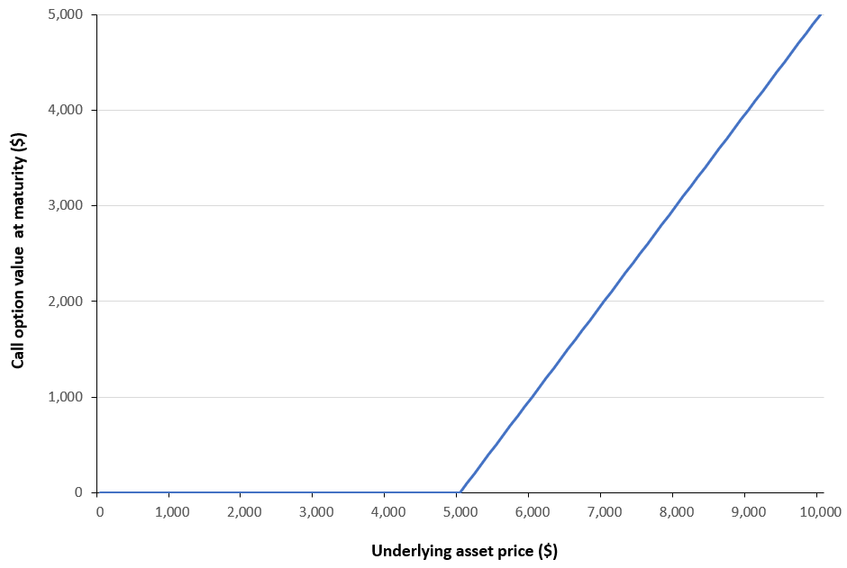
Payoff function
Source: computation by the author.

Call option value

While the value of an option is known at maturity (being determined by its payoff function), its value at any earlier time prior to maturity, and in particular at issuance, is not directly observable. Consequently, a valuation model is required to determine the option’s price at those earlier dates.

The Black–Scholes–Merton model is formulated as a stochastic partial differential equation and the solution to the partial differential equation (PDE) gives the BSM formula for the value of the option.

For a European-style call option, the call option value at issuance is given by the following formula:

Formula for the call option value according to the BSM model

with

Formula for the call option value according to the BSM model

Where the notations are as follows:

C₀= Call option value at issuance (time 0) based on the Black-Scholes-Merton model
K = Strike price (exercise price)
T = Time to expiration
S₀ = Current underlying price (time 0)
r = Risk-free interest rate
σ = Volatility of the underlying asset returns
N(·) = Cumulative distribution function of the standard normal distribution

Figure 2 below illustrates the call option value as a function of the underlying asset price. The example considers a European call written on the S&P 500 index, with a strike price of $5,000 and a time to maturity of 30 days. The current price of the underlying index is $6,000, and the risk-free interest rate is set at 3.79% corresponding to the 1-month U.S. Treasury yield, and the volatility is assumed to be 15%.

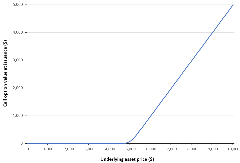
Figure 2. Call option value as a function of the underlying asset price.

Source: computation by the author (BSM model).

Option and volatility

In the Black–Scholes–Merton model, the value of a European call or put option is a monotonically increasing function of volatility. Higher volatility increases the probability of finishing in-the-money while losses remain limited to the option premium, resulting in a strictly positive vega (the first derivative of the option value with respect to volatility) for both calls and puts.

As volatility approaches zero, the option value converges to its intrinsic value, forming a lower bound. With increasing volatility, option values rise toward a finite upper bound equal to the underlying price for calls (and bounded by the strike for puts). An inflection point occurs where volga (the second derivative of the option value with respect to volatility) changes sign: at this point vega is maximized (at-the-money) and declines as the option becomes deep in- or out-of-the-money or as time to maturity decreases.

The upper limit and the lower limit for the call option value function is given below (Hull, 2015, Chapter 11).

Formula for upper and lower limits of the option price

Figure 3 below illustrates the value of a European call option as a function of the underlying asset’s price volatility. The example considers a European call written on the S&P 500 index, with a strike price of $5,000 and a time to maturity of 30 days. The current price of the underlying index is $6,000, and the risk-free interest rate is set at 3.79% corresponding to the 1-month U.S. Treasury yield. A deliberately wide (and economically unrealistic) range of volatility values is employed in order to highlight the theoretical limits of option prices: as volatility tends to infinity, the option value converges to an upper bound ($6,000 in our example), while as volatility approaches zero, the option value converges to a lower bound $1,015.51).

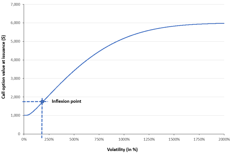
Figure 3. Call option value as a function of price volatility

Source: computation by the author (BSM model).

Volatility: the unobservable parameter of the model

When we think of options, the basic equation to remember is “Option = Volatility”. Unlike stocks or bonds, options are not primarily quoted in monetary units (dollars or euros), but rather in terms of implied volatility, expressed as a percentage.

Volatility is not directly observable in financial markets. It is an unobservable (latent) parameter of the pricing model, inferred endogenously from observed option prices through an inversion of the valuation formula given by the BSM model. As a result, option markets are best interpreted as markets for volatility rather than markets for prices.

Out of the five essential parameters of the Black-Scholes-Merton model listed above, the volatility parameter is the unobservable parameter as it is the future fluctuation in price of the underlying asset over the remaining life of the option from the time of observation. Since future volatility cannot be directly observed, practitioners use the inverse of the BSM model to estimate the market’s expectation of this volatility from option market prices, referred to as implied volatility.

Implied Volatility

In practice, implied volatility is the volatility parameter that when input into the Black-Scholes-Merton formula yields the market price of the option and represents the market’s expectation of future volatility.

Calculating Implied volatility

The BSM model maps five input variables (S, K, r, T, σ_implied) to a single output variable uniquely: the call option value (Price), such that it’s a bijective function. When the market call option price (C_BSM) is known, we invert this relationship using (S, K, r, T, C_BSM) as inputs to solve for the implied volatility, σ_implied.

Formula for implied volatility

Newton-Raphson Method

As there is no closed form solution to calculate implied volatility from the market price, we need a numerical method such as the Newton–Raphson method to compute it. This involves finding the volatility for which the Black–Scholes–Merton option value C_BSM equals the observed market option price C_Market.

We define the function f as the difference between the call option value given by the BSM model and the observed market price of the call option:

Function for the Newton-Raphson method.

Where x represents the unknown variable (implied volatility) to find and C_Market is considered as a constant in the Newton–Raphson method.

Using the Newton-Raphson method, we can iteratively estimate the root of the function, until the difference between two consecutive estimations is less than the tolerance level (ε).

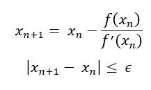
Formula for the iterations in the Newton-Raphson method

In practice, the inflexion point (Tankov, 2006) is taken as the initial guess, because the function f(x) is monotonic, so for very large or very small initial values, the derivative becomes extremely small (see Figure 3), causing the Newton–Raphson update step to overshoot the root and potentially diverge. Selecting the inflection point also minimizes approximation error, as the second derivative of the function at this point is approximately zero, while the first derivative remains non-zero.

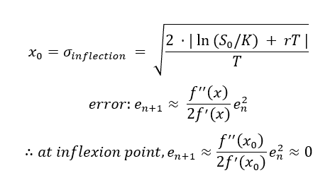
Formula for calculating the volatility at inflexion point.

Where σ_inflection is the volatility at the inflection point.

Figure 4 below illustrates how implied volatility varies with the call option price for different values of the market price (computed using the Newton–Raphson method). As before, the example considers a European call written on the S&P 500 index, with a strike price of $5,000 and a time to maturity of 30 days. The current level of the underlying index is $6,000, and the risk-free interest rate is set at 3.79% corresponding to the 1-month U.S. Treasury yield.

Figure 4. Implied volatility vs. Call Option value
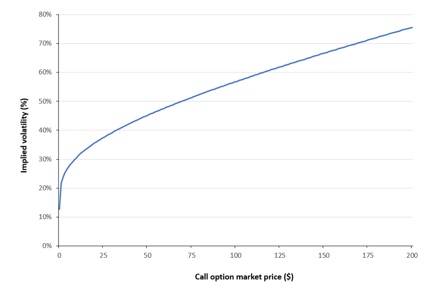
Implied volatility as a function of call option price
Source: computation by the author.

You can download the Excel file provided below, which contains the calculations and charts illustrating the payoff function, the option price as a function of the underlying asset’s price, the option price as a function of volatility, and the implied volatility as a function of the option price.

You can download the Python code provided below, to calculate the price of a European-style call or put option and calculate the implied volatility from the option market price (BSM model). The Python code uses several libraries.

Alternatively, you can download the R code below with the same functionality as in the Python file.

Why should I be interested in this post?

The seminal Black–Scholes–Merton model was originally developed to price European options. Over time, it has been extended to accommodate a wide range of derivatives, including those based on currencies, commodities, and dividend-paying stocks. As a result, the model is of fundamental importance for anyone seeking to understand the derivatives market and to compute implied volatility as a measure of risk.

Useful resources

Academic research

Black F. and M. Scholes (1973) The pricing of options and corporate liabilities. Journal of Political Economy, 81(3), 637–654.

Merton R.C. (1973) Theory of rational option pricing. The Bell Journal of Economics and Management Science, 4(1), 141–183.

Hull J.C. (2022) Options, Futures, and Other Derivatives, 11th Global Edition, Chapter 15 – The Black–Scholes–Merton model, 338–365.

Cox J.C. and M. Rubinstein (1985) Options Markets, First Edition, Chapter 5 – An Exact Option Pricing Formula, 165-252.

Tankov P. (2006) Calibration de Modèles et Couverture de Produits Dérivés (Model calibration and derivatives hedging), Working Paper, Université Paris-Diderot. Available at https://cel.hal.science/cel-00664993/document.

About the BSM model

The Nobel Prize Sveriges Riksbank Prize in Economic Sciences in Memory of Alfred Nobel 1997

Harvard Business School Option Pricing in Theory & Practice: The Nobel Prize Research of Robert C. Merton

Other

NYU Stern Volatility Lab Volatility analysis documentation.

About the author

The article was written in December 2025 by Saral BINDAL (Indian Institute of Technology Kharagpur, Metallurgical and Materials Engineering, 2024-2028 & Research assistant at ESSEC Business School).

▶ Read all posts written by Saral BINDAL.

Historical Volatility

December 20, 2025December 14, 2025 by Saral BINDAL

In this article, Saral BINDAL (Indian Institute of Technology Kharagpur, Metallurgical and Materials Engineering, 2024-2028 & Research Assistant at ESSEC Business School) explains the concept of historical volatility used in financial markets to represent and measure the changes in asset prices.

Introduction

Volatility in financial markets refers to the degree of variation in an asset’s price or returns over time. Simply put, an asset is considered highly volatile when its price experiences large upward or downward movements, and less volatile when those movements are relatively small. Volatility plays a central role in finance as an indicator of risk and is widely used in various portfolio and risk management techniques.

In practice, the concept of volatility can be operationalized in different ways: historical volatility and implied volatility. Traders and analysts use historical volatility to understand an asset’s past performance and implied volatility as a forward-looking measure of upcoming uncertainties in the market.

Historical volatility measures the actual variability of an asset’s price over a past period, calculated as the standard deviation of its historical returns. Computed over different periods (say a month), historical volatility allows investors to identify trends in volatility and assess how an asset has reacted to market conditions in the past.

Practical Example: Analysis of the S&P 500 Index

Let us consider the S&P 500 index as an example of the calculation of volatility.

Prices

Figure 1 below illustrates the daily closing price of the S&P 500 index over the period from January 2020 to December 2025.

Figure 1. Daily closing prices of the S&P 500 index (2020-2025).

Source: computation by the author.

Returns

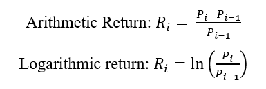
Returns are the percentage gain or loss on the asset’s investment and are generally calculated using one of two methods: arithmetic (simple) or logarithmic (continuously compounded).

Returns Formulas

Where R_i represents the rate of return, and P_i denotes the asset’s price at a given point in time.

The preference for logarithmic returns stems from their property of time-additivity, which simplifies multi-period calculations (the monthly log return is equal to the sum of the daily log returns of the month, which is not the case for arithmetic return). Furthermore, logarithmic returns align with the geometric mean thereby mathematically capture the effects of compounding, unlike arithmetic return, which can overstate performance in volatile markets.

Distribution of returns

A statistical distribution describes the likelihood of different outcomes for a random variable. It begins with classifying the data as either discrete or continuous.

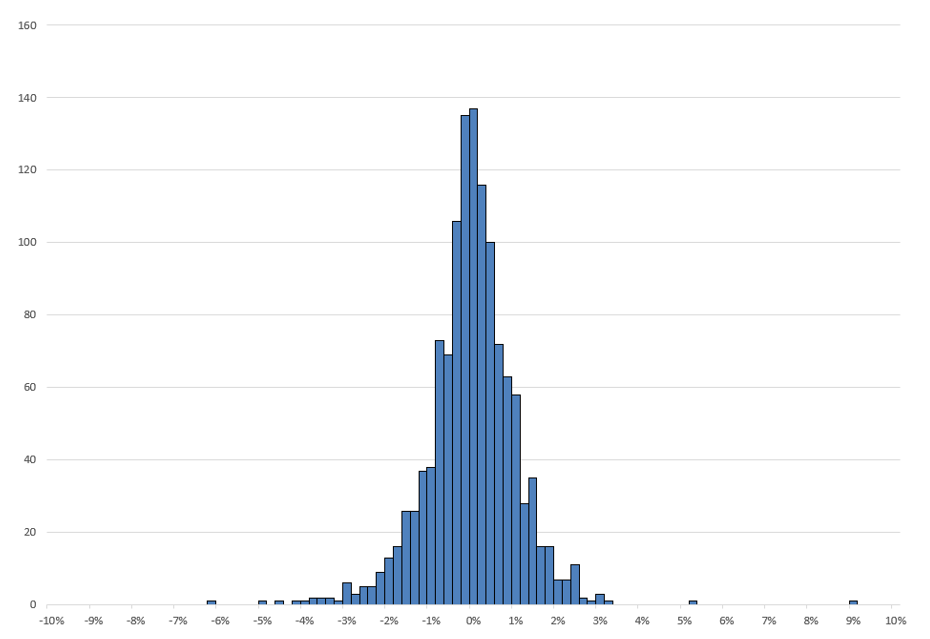
Figure 2 below illustrates the distribution of daily returns for S&P 500 index over the period from January 2020 to December 2025.

Figure 2. Historical distribution of daily returns of the S&P 500 index (2020-2025).

Source: computation by the author.

Standard deviation of the distribution of returns

In real life, as we do not know the mean and standard deviation of returns, these parameters have to be estimated with data.

The estimator for the mean μ, denoted by μ̂, and the estimator for the variance σ², denoted by σ̂², are given by the following formulas:

Formulas for the mean and variance estimators

With the following notations:

R_i = rate of return for the i^th day
μ̂ = estimated mean of the data
σ̂² = estimated variance of the data
n = total number of days for the data

These estimators are unbiased and efficient (note the Bessel’s correction for the standard deviation when we divide by (n–1) instead of n).

Unbiased estimators of the mean and variance

For the distribution of returns in Figure 2, the mean and standard deviation calculated using the formulas above are 0.049% and 1.068%, respectively (in daily units).

Annualized volatility

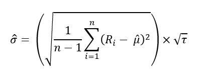
As the usual time frame for human is the year, volatility is often annualized. In order to obtain annual (or annualized) volatility, we scale the daily volatility by the square root of the number of days in that period (τ), as shown below.

Annual Volatility formula

Where  is the number of trading days during the calendar year.

In the U.S. equity market, the annual number of trading days typically ranges from 250 to 255 (252 tradings days in 2025). This variation reflects the holiday calendar: when a holiday falls on a weekday, the exchange closes ; when it falls on a weekend, trading is unaffected. In contrast, the cryptocurrency market has as many trading days as there are calendar days in a year, since it operates continuously, 24/7.

For the S&P 500 index over the period from January 2020 to December 2025, the annualized volatility is given by

S&P500index Annual Volatility formula

Annualized mean

The calculated mean for the 5-year S&P 500 logarithmic returns is also the daily average return for the period. The annualized average return is given by the formula below.

Annualized mean formula

Where τ is the number of trading days during the calendar year.

For the S&P 500 index over the period from January 2020 to December 2025, the annualized average return is given by

Annualized mean formula

If the value of daily average return is much less than 1, annual average return can be approximated as

Annualized mean value

Application: Estimating the Future Price Range of the S&P 500 index

To develop an intuitive understanding of these figures, we can estimate the one-standard-deviation price range for the S&P 500 index over the next year. From the above calculations, we know that the annualized mean return is 12.534% and the annualized standard deviation is 16.953%.

Under the assumption of normally distributed logarithmic returns, we can say approximately with 68% confidence that the value of S&P 500 index is likely to be in the range of:

Upper and lower limits

If the current value of the S&P 500 index is $6,830, then converting these return estimates into price levels gives:

Upper and lower price limits

Based on a 68% confidence interval, the S&P 500 index is likely to trade in the range of $6,526 to $8,838 over the next year.

Historical Volatility

Historical volatility represents the variability of an asset’s returns over a chosen lookback period. The annualized historical volatility is estimated using the formula below.

Historical volatility formula

With the following notations:

σ = Standard deviation
R_i = Return
n = total number of trading days in the period (21 for 1 month, 63 for 3 months, etc.)
τ = Number of trading days in a calendar year

Volatility calculated over different periods must be annualized to a common timeframe to ensure comparability, as the standard convention in finance is to express volatility on an annual basis. Therefore, when working with daily returns, we annualize the volatility by multiplying it by the square root of 252.

For example, for the S&P 500 index, the annualized historical volatilities over the last 1 month, 3 months, and 6 months, computed on December 3, 2025, are 14.80%, 12.41%, and 11.03%, respectively. The results suggest, since the short term (1 month) volatility is higher than medium (3 months) and long term (6 months) volatility, the recent market movements have been turbulent as compared to the past few months, and due to volatility clustering, periods of high volatility often persist, suggesting that this elevated turbulence may continue in the near term.

Unconditional Volatility

Unconditional volatility is a single volatility number using all historical data, which in our example is the entire five years data; It does not account for the fact that recent market behavior is more relevant for predicting tomorrow’s risk than events from past years, implying that volatility changes over time. It is frequently observed that after any sudden boom or crash in the market, as the storm passes away the volatility tends to revert to a constant value and that value is given by the unconditional volatility of the entire period. This tendency is referred to as mean reversion.

For instance, using S&P 500 index data from 2020 to 2025, the unconditional volatility (annualized standard deviation) is calculated to be 16.952%.

Rolling historical volatility

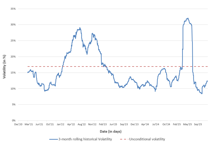
A single volatility number often fails to capture changing market regimes. Therefore, a rolling historical volatility is usually generated to track the evolution of market risk. By calculating the standard deviation over a moving window, we can observe how volatility has expanded or contracted historically. This is illustrated in Figure 3 below for the annualized 3-month historical volatility of the S&P 500 index over the period 2020-2025.

Figure 3. 3-month rolling historical volatility of the S&P500 index (2020-2025).

Source: computation by the author.

In Figure 3, the 3-month rolling historical volatility is plotted along with the unconditional volatility computed over the entire period, calculated using overlapping windows to generate a continuous series. This provides a clear historical perspective, showcasing how the asset’s volatility has fluctuated relative to its long-term average.

For example, during the start of Russia–Ukraine war (February 2022 – August 2022), a noticeable jump in volatility occurred as energy and food prices surged amid fears of supply chain disruptions, given that Russia and Ukraine are major exporters of oil, natural gas, wheat, and other commodities.

The rolling window can be either overlapping or non-overlapping, resulting in continuous or discrete graphs, respectively. Overlapping windows shift by one day, creating a smooth and continuous volatility series, whereas non-overlapping windows shift by one time period, producing a discrete series.

You can download the Excel file provided below, which contains the computation of returns, their historical distribution, the unconditional historical volatility, and the 3-month rolling historical volatility of the S&P 500 index used in this article.

You can download the Python code provided below, which contains the computation of returns, first four moments of the distribution, and experiment with the x-month rolling historical volatility function to visualize the evolution of historical volatility over time.

Alternatively, you can download the R code below with the same functionality as in the Python file.

Alterative measures of volatility

We now mention a few other ways volatility can be measured: Parkinson volatility, Implied volatility, ARCH model, and stochastic volatility model.

Parkinson volatility

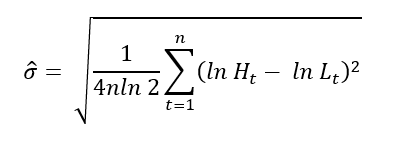
The Parkinson model (1980) uses the highest and lowest prices during a given period (say a month) for the purpose of measurement of volatility. This model is a high-low volatility measure, based on the difference between the maximum and minimum prices observed during a certain period.

Parkinson volatility is a range-based variance estimator that replaces squared returns with the squared high–low log price range, scaled to remain unbiased. It assumes a driftless (expected growth rate of the stock price equal to zero) geometric Brownian motion, it is five times more efficient than close-to-close returns because it accounts for fluctuation of stock price within a day.

For a sample of n observations (say days), the Parkinson volatility is given by

Parkinson Volatility formula

where:

H_t is the highest price on period t
L_t is the lowest price on period t

Implied volatility

Implied Volatility (IV) is the level of volatility for the underlying asset that, when plugged into an option pricing model such as Black–Scholes–Merton, makes the model’s theoretical option price equal to the option’s observed market price.

It is a forward looking measure because it reflects the market’s expectation of how much the underlying asset’s price is likely to fluctuate over the remaining life of the option, rather than how much it has moved in the past.

The Chicago Board Options Exchange (CBOE), a leading global financial exchange operator provides implied volatility indices like the VIX and Implied Correlation Index, measuring 30-day expected volatility from SPX options. These are used by traders to gauge market fear, speculate via futures/options/ETPs, hedge equity portfolios and manage risk during volatility spikes.

ARCH model

Autoregressive Conditional Heteroscedasticity (ARCH) models address time-varying volatility in time series data. Introduced by Engle in 1982, ARCH models look at the size of past shocks to estimate how volatile the next period is likely to be. If recent movements were big, the model expects higher volatility; if they were small, it expects lower volatility justifying the idea of volatility clustering. Originally applied to inflation data, this model has been widely used in to model financial data.

ARCH model capture volatility clustering, which refers to an observation about how volatility behaves in the short term, a large movement is usually followed by another large movement, thus volatility is predictable in the short term. Historical volatility gives a short-term hint of the near future changes in the market because recent noise often continues.

Generalized Autoregressive Conditional Heteroscedasticity (GARCH) extends ARCH by past predicted volatility, not just past shocks, as refined by Bollerslev in 1986 from Engle’s work. Both of these methods are more accurate methods to forecast volatility than what we had discussed as they account for the time varying nature of volatility.

Stochastic volatility models

In practice, volatility is time-varying: it exhibits clustering, persistence, and mean reversion. To capture these empirical features, stochastic volatility (SV) models treat volatility not as a constant parameter but as a stochastic process jointly evolving with the asset price. Among these models, the Heston (1993) specification is one of the most influential.

The Heston model assumes that the asset price follows a diffusion process analogous to geometric Brownian motion, while the instantaneous variance evolves according to a mean-reverting square-root process. Moreover, the innovations to the price and variance processes are correlated, thereby capturing the leverage effect frequently observed in equity markets.

Applications in finance

This section covers key mathematical concepts and fundamental principles of portfolio management, highlighting the role of volatility in assessing risk.

The normal distribution

The normal distribution is one of the most commonly used probability distribution of a random variable with a unimodal, symmetric and bell-shaped curve. The probability distribution function for a random variable X following a normal distribution with mean μ and variance σ² is given by

Normal distribution function

A random variable X is said to follow standard normal distribution if its mean is zero and variance is one.

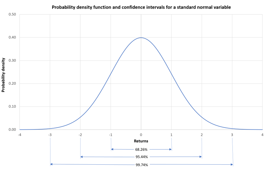
The figure below represents the confidence intervals, showing the percentage of data falling within one, two, and three standard deviations from the mean.

Figure 4. Probability density function and confidence intervals for a standard normal varaible.
Standard normal distribution” width=
Source: computation by the author

Brownian motion

Robert Brown first observed Brownian motion was as the erratic and random movement of pollen particles suspended in water due to constant collision with water molecules. It was later formulated mathematically by Norbert Wiener and is also known as the Wiener process.

The random walk theory suggests that it’s impossible to predict future stock prices as they move randomly, and when the timestep of this theory becomes infinitesimally small it becomes, Brownian Motion.

In the context of financial stochastic process, when the market is modeled by the standard Brownian motion, the probability distribution function of the future price is a normal distribution, whereas when modeled by Geometric Brownian Motion, the future prices are said to be lognormally distributed. This is also called the Brownian Motion hypothesis on the movement of stock prices.

The process of a standard Brownian motion is given by:

Standard Brownian motion formula.

The process of a geometric Brownian motion is given by:

Geometric Brownian motion formula.

Where, dS_t is the change in asset price in continuous time dt, dX_t is a random variable from the normal distribution (N (0, 1)) or Wiener process at a time t, σ represents the price volatility, and μ represents the expected growth rate of the asset price, also known as the ‘drift’.

Modern Portfolio Theory (MPT)

Modern Portfolio Theory (MPT), developed by Nobel Laureate, Harry Markowitz, in the 1950s, is a framework for constructing optimal investment portfolios, derived from the foundational mean-variance model.

The Markowitz mean–variance model suggests that risk can be reduced through diversification. It proposes that risk-averse investors should optimize their portfolios by selecting a combination of assets that balances expected return and risk, thereby achieving the best possible return for the level of risk they are willing to take. The optimal trade-off curve between expected return and risk, commonly known as the efficient frontier, represents the set of portfolios that maximizes expected return for each level of standard deviation (risk).

Capital Asset Pricing Model (CAPM)

The Capital Asset Pricing Model (CAPM) builds on the model of portfolio choice developed by Harry Markowitz (1952), stated above. CAPM states that, assuming full agreement on return distributions and either risk-free borrowing/lending or unrestricted short selling, the value-weighted market portfolio of risky assets is mean-variance efficient, and expected returns are linear in the market beta.

The main result of the CAPM is a simple mathematical formula that links the expected return of an asset to its risk measured by the beta of the asset:

CAPM formula

Where:

E(R_i) = expected return of asset i
R_f = risk-free rate
β_i = measure of the risk of asset i
E(R_m) = expected return of the market
E(R_m) − R_f = market risk premium

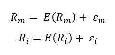
CAPM recognizes that an asset’s total risk has two components: systematic risk and specific risk, but only systematic risk is compensated in expected returns.

Returns decomposition fromula.

Where the realized (actual) returns of the market (R_m) and the asset (R_i) exceed their expected values only because of consideration of systematic risk (ε).

Decomposition of risk.
Decompositionion of risk

Systematic risk is a macro-level form of risk that affects a large number of assets to one degree or another, and therefore cannot be eliminated. General economic conditions, such as inflation, interest rates, geopolitical risk or exchange rates are all examples of systematic risk factors.

Specific risk (also called idiosyncratic risk or unsystematic risk), on the other hand, is a micro-level form of risk that specifically affects a single asset or narrow group of assets. It involves special risk that is unconnected to the market and reflects the unique nature of the asset. For example, company specific financial or business decisions which resulted in lower earnings and affected the stock prices negatively. However, it did not impact other asset’s performance in the portfolio. Other examples of specific risk might include a firm’s credit rating, negative press reports about a business, or a strike affecting a particular company.

Why should I be interested in this post?

Understanding different measures of volatility, is a pre-requisite to better assess potential losses, optimize portfolio allocation, and make informed decisions to balance risk and expected return. Volatility is fundamental to risk management and constructing investment strategies.

Useful Resources

Academic research

Bollerslev, T. (1986). Generalized Autoregressive Conditional Heteroskedasticity, Journal of Econometrics, 31(3), 307–327.

Engle, R. F. (1982). Autoregressive Conditional Heteroscedasticity with Estimates of the Variance of United Kingdom Inflation, Econometrica, 50(4), 987–1007.

Fama, E. F., & French, K. R. (2004). The Capital Asset Pricing Model: Theory and Evidence, Journal of Economic Perspectives, 18(3), 25–46.

Heston, S. L. (1993). A Closed-Form Solution for Options with Stochastic Volatility with Applications to Bond and Currency Options, The Journal of Finance, 48(3), 1–24.

Markowitz, H. M. (1952). Portfolio Selection, The Journal of Finance, 7(1), 77–91.

Parkinson, M. (1980). The extreme value method for estimating the variance of the rate of return. Journal of Business, 53(1), 61–65.

Sharpe, W. F. (1964). Capital Asset Prices: A Theory of Market Equilibrium under Conditions of Risk, The Journal of Finance, 19(3), 425–442.

Tsay, R. S. (2010). Analysis of financial time series, John Wiley & Sons.

Other

NYU Stern Volatility Lab Volatility analysis documentation.

Extreme Events in Finance Risk maps: extreme risk, risk and performance.

About the author

The article was written in December 2025 by Saral BINDAL (Indian Institute of Technology Kharagpur, Metallurgical and Materials Engineering, 2024-2028 & Research Assistant at ESSEC Business School).

▶ Read all articles by Saral BINDAL.

Pricing Weather Risk: How to Value Agricultural Derivatives with Climate-Based Volatility Inputs

May 29, 2025 by Mathias DUMONT

In this article, Mathias DUMONT (ESSEC Business School, Global Bachelor in Business Administration (GBBA), 2022-2026) explains how weather risk impacts the pricing of agricultural derivatives like futures and options, and how climate-based data can be integrated into stochastic pricing models. Combining academic insights and practical examples, including a mini-case from the SimTrade Blé de France simulation, the article illustrates adjustments to models such as the Black-Scholes-Merton model for temperature and rainfall variables in valuing agricultural contracts.

Introduction

Extreme weather has always been a critical factor in agriculture, but climate change is amplifying the frequency and severity of these events. From prolonged droughts to unseasonal floods, weather shocks can send crop yields and commodity prices on wild rides. This rising uncertainty has given birth to weather derivatives – financial instruments designed to hedge weather-related risks – and has made volatility forecasting a key challenge in pricing agricultural contracts. In fact, as businesses grapple with climate volatility, trading volume in weather derivatives has surged. CME Group saw a 260% increase last year (CME Group, 2023). The question for traders and risk managers is: how do we quantitatively factor weather risk into the pricing of futures and options on crops like wheat and corn?

Weather Risk and Agricultural Markets

Weather directly affects crop supply. A bumper harvest following ideal weather can flood the market and depress prices, whereas a drought or frost can decimate yields and trigger price spikes. These supply swings translate into volatility for agricultural commodity markets. For example, during the U.S. drought of 2012, corn prices skyrocketed, and the implied volatility of corn futures jumped by over 14 percentage points within a month, reaching ~49% in mid-July. Such surges reflect the market rapidly repricing risk as participants absorb new climate information (in this case, worsening crop prospects). Seasonal patterns are also evident: harvest seasons tend to coincide with higher price volatility because that’s when weather uncertainty is at its peak. Studies show that harvesting cycles create predictable seasonal volatility patterns in crop markets – when a critical growth period is underway, any shift in rainfall or temperature forecasts can send prices swinging.

Beyond affecting supply quantity, weather can influence crop quality (e.g., excessive rain can spoil grain quality) and even logistic costs (flooded transport routes, etc.), further feeding into prices. The interconnected global nature of agriculture means a drought in one region can reverberate worldwide. As noted in the SimTrade Blé de France case, weather conditions in France influence the quantity and quality of wheat the company harvests, while weather conditions around the world influence the international wheat price. In the Blé de France simulation (which models a French wheat producer’s stock), participants see how news of floods or droughts translate into stock price moves. For instance, the company might project a 7-million-ton wheat harvest, but analysts’ forecasts range from 6.5 to 7.2 Mt – with the realized level highly weather-dependent in the final weeks of the season. A poor weather turn not only shrinks the crop but boosts global wheat prices, creating a complex revenue impact on the firm. This mini-case underlines that weather risk entails both volume uncertainty and price uncertainty, a double-whammy for agricultural firms and their investors.

Case Study: Weather Shocks in Wheat Markets

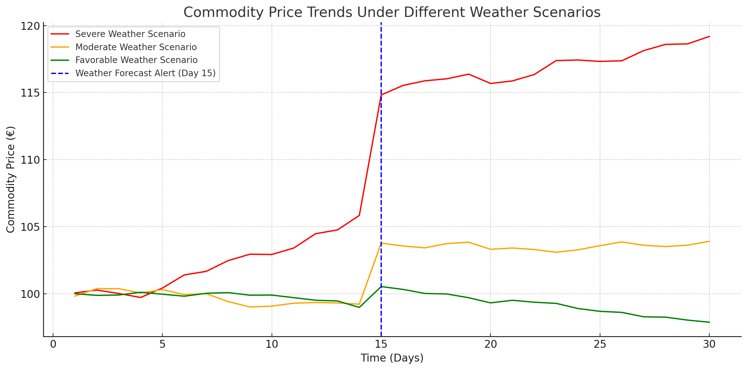
To illustrate the impact of weather risk on commodity pricing, consider three simulated scenarios for an upcoming wheat growing season: (1) **Favorable weather**, (2) **Moderate conditions**, and (3) **Severe weather** such as drought. Each scenario generates a distinct price trajectory in the wheat market. Under favorable weather, prices tend to remain stable or decline slightly, particularly at harvest, due to strong yields and potential oversupply. In moderate conditions, prices may rise modestly as the market adjusts to balanced supply and demand. In contrast, severe weather triggers early price rallies as concerns about yield shortfalls emerge, followed by sharp spikes once crop damage becomes evident. For producers and traders, anticipating these divergent price paths is essential for pricing contracts, managing risk exposure, and structuring hedging strategies effectively.

Figure 1. Simulated commodity price paths under three weather scenarios.
Simulated Price Paths
Source: Author’s simulation.

Figure 1. shows the simulation of commodity price paths under three weather scenarios: severe weather (red), moderate weather (orange), and favorable weather (green). A mid-season weather forecast alert (Day 15) triggers a shift in market expectations, causing price divergence. This simulation illustrates how weather shocks and forecasts impact commodity pricing through volatility and revised yield expectations.

From a risk management perspective, tools exist to handle these contingencies. Farmers or firms concerned about catastrophic weather can turn to weather derivatives for protection. Weather derivatives are financial contracts (often based on indexes like temperature or rainfall levels) that pay out based on specific weather outcomes, allowing businesses to offset losses caused by adverse conditions. They have been used by a wide range of players – from utilities hedging warm winters, to breweries hedging late frosts. These instruments can be customized over-the-counter or traded on exchanges. Notably, CME Group lists standardized weather futures and options tied to indices such as heating degree days (HDD) and cooling degree days (CDD) for various cities. The existence of such contracts means that even when commodity producers cannot fully insure their crop yield, they might hedge certain aspects of weather risk (like an unusually hot summer) via financial markets. In our context, a wheat farmer worried about drought could, say, buy a weather option that pays off if rainfall falls below a threshold, providing funds when their crop output (and thus futures position) suffers.

Climate-Based Volatility in Derivatives Pricing

How can weather uncertainty be incorporated into derivative pricing models? Classic option pricing, such as the Black-Scholes-Merton model, assumes a fixed volatility for the underlying asset’s returns. For agricultural commodities, that volatility is anything but constant – it ebbs and flows with the weather and seasonal progress. Practitioners thus often use stochastic volatility models or at least adjust the volatility input over time. For example, one might use higher volatility estimates during the crop’s growing season and lower volatility post-harvest when output is known. This practice parallels how equity traders anticipate higher volatility in stock prices ahead of major earnings or profit announcements, and lower volatility after the announcement of profits by the firm.

Like companies facing performance surprises, weather shocks inject information asymmetry into the market, which must be priced into the option premiums. This aligns with the observed Samuelson effect, where futures contracts on commodities tend to have higher volatility when they are near maturity (coinciding with harvest uncertainty).

Market prices of options themselves reflect these expectations. When a looming weather event is expected to cause turmoil, options premiums will rise. The metric capturing this is implied volatility – the volatility level implied by current option prices. Implied vol is essentially forward-looking and will jump if traders foresee choppy waters ahead. Empirical evidence shows that extreme weather forecasts translate into higher implied vols for crop options. In 2012, as drought fears intensified, corn option implied volatility spiked (alongside futures prices). Conversely, once a forecasted drought started being relieved by rains, implied volatility eased off, signaling that some uncertainty had been resolved. A recent study also found that integrating meteorological data (like rainfall and temperature anomalies) into volatility modeling significantly improves the ability to hedge risk in agricultural markets. In other words, the more information we feed into our models about the climate, the more accurately we can price and hedge these derivatives.

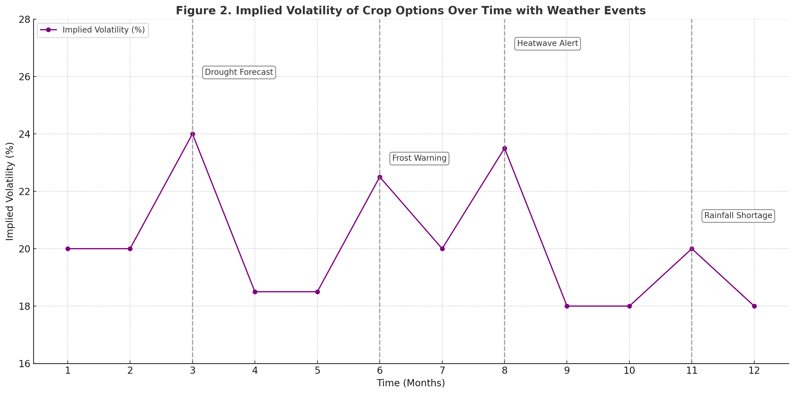
Figure 2. Implied Volatility of Crop Options Over Time with Weather Events
Line chart showing implied volatility of crop options over 12 months with spikes linked to weather events
Source: Author’s simulation.

This simulation illustrates the evolution of implied volatility over a 12-month crop cycle. Forecasted climate events—drought (Month 3), frost (Month 6), heatwave (Month 8), and rainfall shortage (Month 11)—lead to moderate but distinct volatility spikes. As uncertainty resolves, volatility returns to baseline.

One practical approach to pricing under climate uncertainty is to use scenario-based or simulation-based models. Instead of assuming a single volatility number, an analyst can simulate thousands of possible weather outcomes (perhaps using historical climate data or meteorological forecast models) and the corresponding price paths for the commodity. Each simulated price path yields a payoff for the derivative (e.g. an option’s payoff at expiration), and by averaging those payoffs (and discounting appropriately), one can derive a weather-adjusted theoretical price. This Monte Carlo style approach effectively treats weather as an external random factor influencing the commodity’s drift and volatility. It’s particularly useful for complex derivatives or when the payoff depends explicitly on weather indices (such as a derivative that pays out if rainfall is below X mm).

When the derivative’s underlying is the commodity itself (e.g. a corn futures option), traditional risk-neutral pricing arguments still apply, but the challenge is forecasting volatility. Traders often adjust the volatility smile/skew on agricultural options to account for asymmetric weather risks – for instance, if a drought can cause a much bigger upside move than a rainy season can cause a downside move, call options might embed a higher implied volatility (reflecting that upside risk of price spikes). This is observed in practice as well; extreme weather events can distort the implied volatility “skew” of crop options, as out-of-the-money calls become more sought after as disaster insurance.

In contrast, if the derivative’s underlying is a pure weather index (say an option on cumulative rainfall), then pricing becomes more complex because the underlying (rainfall) is not a tradable asset. In such cases, the Black-Scholes-Merton formula is not directly applicable. Instead, pricing relies on actuarial or risk-neutral methodologies that incorporate a market price of risk for weather. For example, one method is to estimate the probability distribution of the weather index from historical data, then add a risk premium to account for investors’ risk aversion to weather variability, and discount expected payoffs accordingly. Another method uses “burn analysis” – taking historical weather outcomes and the associated financial losses/gains had the derivative been in place, to gauge a fair premium. Academic research has proposed models ranging from modified Black-Scholes-Merton-type formulas for rainfall (with adjustments for the non-tradability) to advanced statistical models (e.g. Ornstein-Uhlenbeck processes with seasonality for temperature indices. The key takeaway is that whether it’s directly in commodity options or in dedicated weather derivatives, climate factors force us to go beyond textbook models and embrace more dynamic, data-driven pricing techniques.

Why should I be interested in this post?

For an ESSEC student or a young finance professional, this topic sits at the intersection of finance and real-world impact. Understanding weather risk in markets is not just about farming – it’s about how big data and climate science are increasingly intertwined with financial strategy. Agricultural commodities remain a cornerstone of the global economy, and volatility in these markets can affect food prices, inflation, and even economic stability in various countries. By grasping how to value derivatives with climate-based volatility inputs, you are gaining insight into a growing niche of finance that deals with sustainability and risk management. Moreover, the skills involved – scenario analysis, simulation modeling, blending of economic and scientific data – are highly transferable to other domains (think energy markets or any sector where uncertainty reigns). In a world facing climate change, expertise in weather-related financial products could open career opportunities in commodity trading desks, insurance/reinsurance firms, or specialized hedge funds. Ultimately, this post encourages you to think creatively and interdisciplinarily: the best hedging or valuation solutions may come from combining financial theory with environmental intelligence.

Useful resources

Chicago Mercantile Exchange (CME) Weather futures and options product information. (Exchange-traded weather derivative contracts on temperature and other indices)

U.S. Energy Information Administration Drought increases price of corn, reduces profits to ethanol producers (2012). (Article discussing the 2012 drought’s impact on corn prices and volatility)

Nature Communications (2024) Financial markets value skillful forecasts of seasonal climate. (Research showing that seasonal climate outlooks have measurable effects on implied volatility and market uncertainty)

Das, S. et al. (2025) Predicting and Mitigating Agricultural Price Volatility Using Climate Scenarios and Risk Models. (Academic study demonstrating the integration of climate data into volatility models and using Black-Scholes to value a government price support as a put option)

Pai, J. & Zheng, Z. (2013) Pricing Temperature Derivatives with a Filtered Historical Simulation Approach. (Discussion of why Black-Scholes is not directly applicable to weather derivatives and alternative pricing approaches)

About the author

The article was written in May 2025 by Mathias DUMONT (ESSEC Business School, Global Bachelor in Business Administration (GBBA), 2022-2026).

Implied Volatility

May 15, 2022 by Jayati WALIA

In this article, Jayati WALIA (ESSEC Business School, Grande Ecole Program – Master in Management, 2019-2022) explains how implied volatility is computed from option market prices and a option pricing model.

Introduction

Volatility is a measure of fluctuations observed in an asset’s returns over a period of time. The standard deviation of historical asset returns is one of the measures of volatility. In option pricing models like the Black-Scholes-Merton model, volatility corresponds to the volatility of the underlying asset’s return. It is a key component of the model because it is not directly observed in the market and cannot be directly computed. Moreover, volatility has a strong impact on the option value.

Mathematically, in a reverse way, implied volatility is the volatility of the underlying asset which gives the theoretical value of an option (as computed by Black-Scholes-Merton model) equal to the market price of that option.

Implied volatility is a forward-looking measure because it is a representation of expected price movements in an underlying asset in the future.

Computation methods for implied volatility

The Black-Scholes-Merton (BSM) model provides an analytical formula for the price of both a call option and a put option.

The value for a call option at time t is given by:

Call option value

The value for a put option at time t is given by:

Put option value

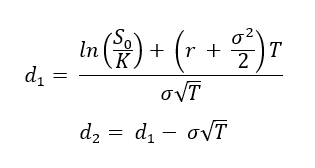
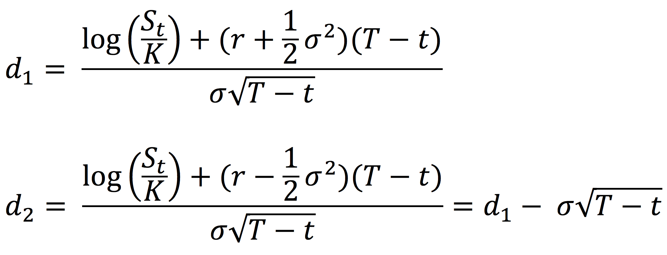
where the parameters d₁ and d₂ are given by:,

call option d1 d2

with the following notations:

S_t : Price of the underlying asset at time t
t: Current date
T: Expiry date of the option
K: Strike price of the option
r: Risk-free interest rate
σ: Volatility of the underlying asset
N(.): Cumulative distribution function for a normal (Gaussian) distribution. It is the probability that a random variable is less or equal to its input (i.e. d₁ and d₂) for a normal distribution. Thus, 0 ≤ N(.) ≤ 1

From the BSM model, both for a call option and a put option, the option price is an increasing function of the volatility of the underlying asset: an increase in volatility will cause an increase in the option price.

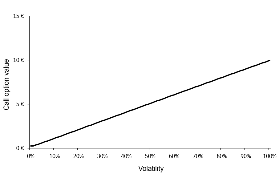
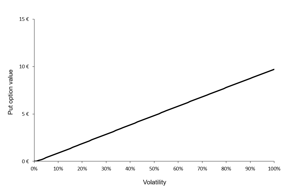
Figures 1 and 2 below illustrate the relationship between the value of a call option and a put option and the level of volatility of the underlying asset according to the BSM model.

Figure 1. Call option value as a function of volatility.

Source: computation by the author (BSM model)

Figure 2. Put option value as a function of volatility.

Source: computation by the author (BSM model)

You can download below the Excel file for the computation of the value of a call option and a put option for different levels of volatility of the underlying asset according to the BSM model.

We can observe that the call and put option values are a monotonically increasing function of the volatility of the underlying asset. Then, for a given level of volatility, there is a unique value for the call option and a unique value for the put option. This implies that this function can be reversed; for a given value for the call option, there is a unique level of volatility, and similarly, for a given value for the put option, there is a unique level of volatility.

The BSM formula can be reverse-engineered to compute the implied volatility i.e., if we have the market price of the option, the market price of the underlying asset, the market risk-free rate, and the characteristics of the option (the expiration date and strike price), we can obtain the implied volatility of the underlying asset by inverting the BSM formula.

Example

Consider a call option with a strike price of 50 € and a time to maturity of 0.25 years. The market risk-free interest rate is 2% and the current price of the underlying asset is 50 €. Thus, the call option is ‘at-the-money’. If the market price of the call option is equal to 2 €, then the associated level of volatility (implied volatility) is equal to 18.83%.

You can download below the Excel file below to compute the implied volatility given the market price of a call option. The computation uses the Excel solver.

Volatility smile

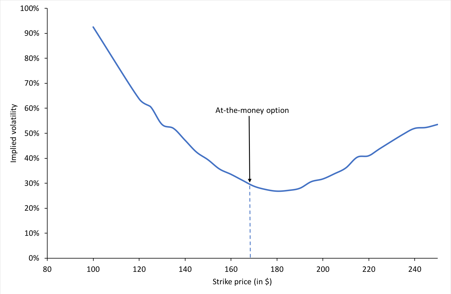
Volatility smile is the name given to the plot of implied volatility against different strikes for options with the same time to maturity. According to the BSM model, it is a horizontal straight line as the model assumes that the volatility is constant (it does not depend on the option strike). However, in practice, we do not observe a horizontal straight line. The curve may be in the shape of the alphabet ‘U’ or a ‘smile’ which is the usual term used to refer to the observed function of implied volatility.

Figure 3 below depicts the volatility smile for call options on the Apple stock on May 13, 2022.

Figure 3. Volatility smile for call options on Apple stock.
Apple volatility smile
Source: Computation by author.

We can also observe that the for a specific time to maturity, the implied volatility is minimum when the option is at-the-money.

Volatility surface

An essential assumption of the BSM model is that the returns of the underlying asset follow geometric Brownian motion (corresponding to log-normal distribution for the price at a given point in time) and the volatility of the underlying asset price remains constant over time until the expiration date. Thus theoretically, for a constant time to maturity, the plot of implied volatility and strike price would be a horizontal straight line corresponding to a constant value for volatility.

Volatility surface is obtained when values for implied volatilities are calculated for options with different strike prices and times to maturity.

CBOE Volatility Index

The Chicago Board Options Exchange publishes the renowned Volatility Index (also known as VIX) which is an index based on the implied volatility of 30-day option contracts on the S&P 500 index. It is also called the ‘fear gauge’ and it is a representation of the market outlook for volatility for the next 30 days.

Useful resources

Academic articles

Black F. and M. Scholes (1973) “The Pricing of Options and Corporate Liabilities” The Journal of Political Economy, 81, 637-654.

Dupire B. (1994). “Pricing with a Smile” Risk Magazine 7, 18-20.

Merton R.C. (1973) “Theory of Rational Option Pricing” Bell Journal of Economics, 4, 141–183.

Business

CBOE Volatility Index (VIX)

CBOE VIX tradable products

About the author

The article was written in May 2022 by Jayati WALIA (ESSEC Business School, Grande Ecole Program – Master in Management, 2019-2022).

Standard deviation

December 11, 2025December 9, 2021 by Jayati WALIA

In this article, Jayati WALIA (ESSEC Business School, Grande Ecole Program – Master in Management, 2019-2022) presents an overview of standard deviation and its use in financial markets.

Definition

The standard deviation is a measure that indicates how much data scatter around the mean. The idea is to measure how an observation deviates from the mean on average./p>

Mathematical formulae

The first step to compute the standard deviation is to compute the mean. Considering a variable X, the arithmetic mean of a data set with N observations, X₁, X₂ … X_N, is computed as:

img_arithmetic_mean

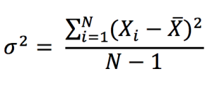
In the data set analysis, we also consider the dispersion or variability of data values around the central tendency or the mean. The variance of a data set is a measure of dispersion of data set values from the (estimated) mean and can be expressed as:

variance

Note that in the above formula we divide by N-1 because the mean is not known but estimated (usual case in finance). If the mean is known with certainty (when dealing the whole population not a sample), then we divide by N.

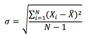
A problem with variance, however, is the difficulty of interpreting it due to its squared unit of measurement. This issue is resolved by using the standard deviation, which has the same measurement unit as the observations of the data set (such as percentage, dollar, etc.). The standard deviation is computed as the square root of variance:

standard deviation

A low value standard deviation indicates that the data set values tend to be closer to the mean of the set and thus lower dispersion, while a high standard deviation indicates that the values are spread out over a wider range indication higher dispersion.

Measure of volatility

For financial investments, the X variable in the above formulas would correspond to the return on the investment computed on a given period of time. We usually consider the trade-off between risk and reward. In this context, the reward corresponds to the expected return measured by the mean, and the risk corresponds to the standard deviation of returns.

In financial markets, the standard deviation of asset returns is used as a statistical measure of the risk associated with price fluctuations of any particular security or asset (such as stocks, bonds, etc.) or the risk of a portfolio of assets (such as mutual funds, index mutual funds or ETFs, etc.).

Investors always consider a mathematical basis to make investment decisions known as mean-variance optimization which enables them to make a meaningful comparison between the expected return and risk associated with any security. In other words, investors expect higher future returns on an investment on average if that investment holds a relatively higher level of risk or uncertainty. Standard deviation thus provides a quantified estimate of the risk or volatility of future returns.

In the context of financial securities, the higher the standard deviation, the greater is the dispersion between each return and the mean, which indicates a wider price range and hence greater volatility. Similarly, the lower the standard deviation, the lesser is the dispersion between each return and the mean, which indicates a narrower price range and hence lower volatility for the security.

Example: Apple Stock

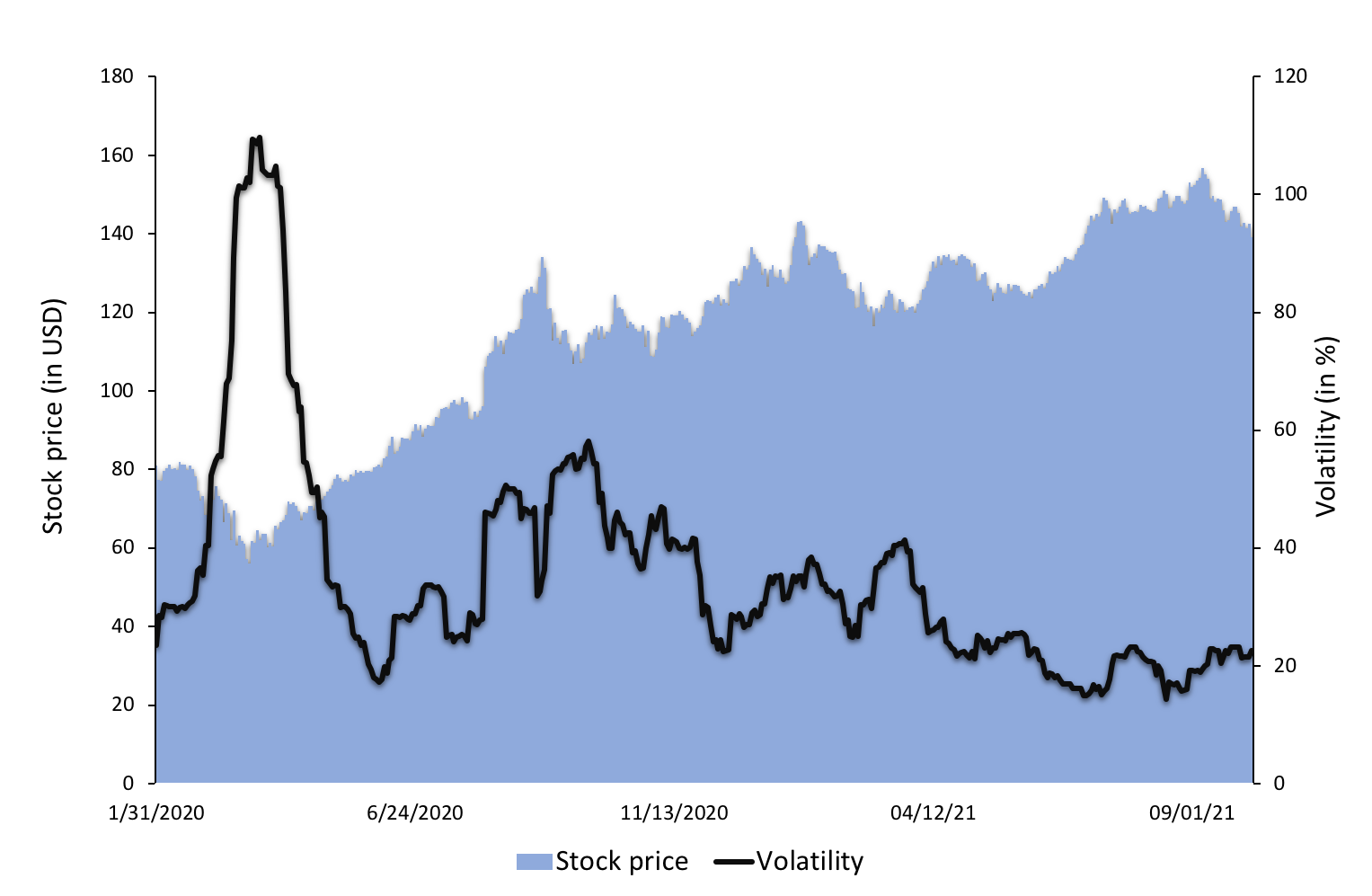
To illustrate the concept of volatility in financial markets, we use a data set of Apple stock prices. At each date, we compute the volatility as the standard deviation of daily stock returns over a rolling window corresponding to the past calendar month (about 22 trading days). This daily volatility is then annualized and expressed as a percentage.

Figure 1. Stock price and volatility of Apple stock.

price and volatility for Apple stock
Source: computation by the author (data source: Bloomberg).

You can download below the Excel file for the calculation of the volatility of stock returns. The data used are for Apple for the period 2020-2021.

Useful resources

Wikipedia Standard Deviation

About the author

The article was written in November 2021 by Jayati WALIA (ESSEC Business School, Grande Ecole Program – Master in Management, 2019-2022).

VIX index

September 12, 2021 by Youssef LOURAOUI

VIX index

In this article, Youssef LOURAOUI (ESSEC Business School, Global Bachelor of Business Administration, 2017-2021) presents the VIX index, which is a financial index that measures the uncertainty in the US equity market.

This article is structured as follows: we begin by defining the grounding notions of the VIX index. We then explain the behavior of this index and its statistical characteristics. We finish by presenting its practical usage in financial markets.

Definition

The CBOE Volatility Index, abbreviated “VIX”, is a measure of the expected S&P 500 index movement calculated by the Chicago Board Options Exchange (CBOE) from the current trading prices of options written on the S&P 500 index.

Known as Wall Street’s “fear index”, the VIX is closely monitored by a broad range of market players, and its level and pattern have become ingrained in market discussion.

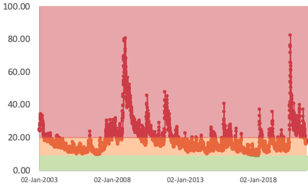
Figure 1 illustrates the evolution of the VIX index for the period from 2003 to 2021.
Figure 1 Historical levels of the VIX index from 2003-2021.

Source: computation by the author (Data source: Thomson Reuters).

VIX values greater than 20 are regarded to be high by market participants. If the VIX is between 12 and 20, it is considered normal; if it is less than 12, it is considered low. As it is the case with other indices, the VIX is computed using the price of a basket of tradable components (in this case, options expiring within the next month or so). The profit or loss that option buyers and sellers realize during the option’s life will depend, among other things, on how significantly the S&P 500’s actual volatility will differ from the implied volatility given by the VIX at the start of the period (S&P Global Research, 2017).

Behavior of the VIX index

Statistical distribution of the S&P500 index returns and VIX level

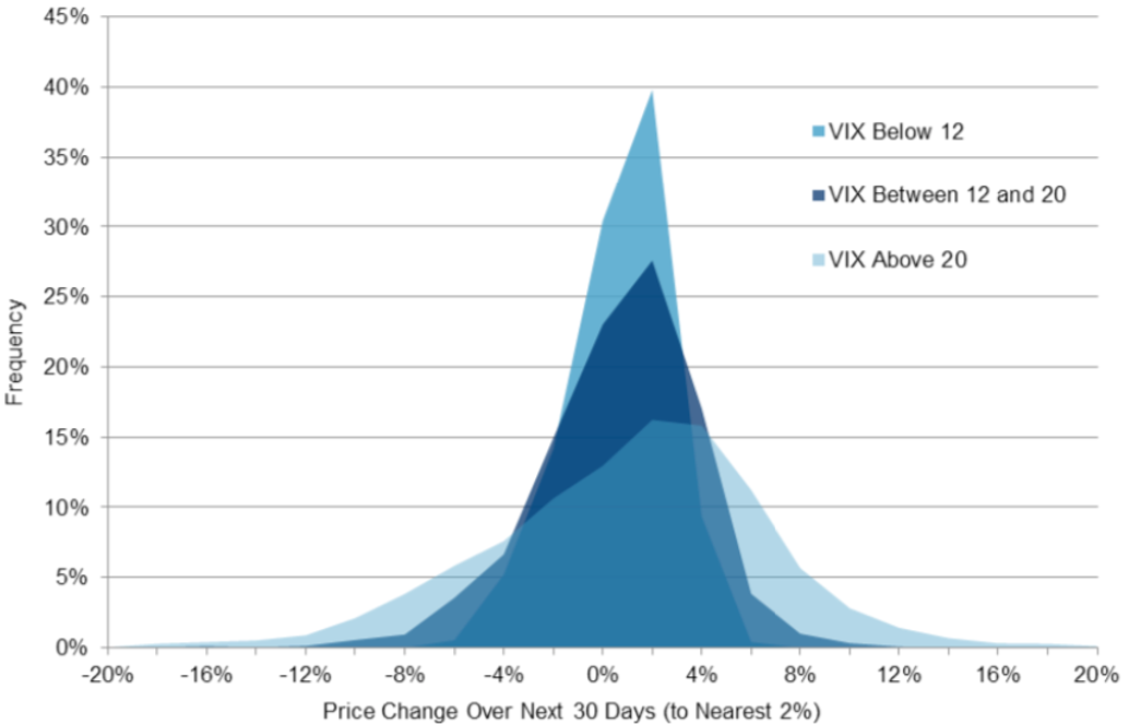
Figure 2 displays the statistical distribution of the price variations in the S&P500 index for different levels of the VIX index The higher the VIX index (by convention, greater than 20), the more severe the distribution tends to be, with negative skewness and high kurtosis indicating heightened volatility in the US market, therefore exacerbating both positive and negative swings. An opposite finding may be made for the VIX level at lower levels (often less than 12), when market swings are less evident due to less skewness and lower kurtosis (S&P Global Research, 2017).

Figure 2. The distribution of 30-day return in the S&P500 index for different VIX index levels.

Source: S&P Global Research (2017).

If the VIX is low, market players may benefit by purchasing options; conversely, if the VIX is high, market participants may profit from selling options. The specific utility of anticipated VIX is that it gives us with a more accurate assessment of whether VIX is high, low, or normal at any point in time (S&P Global Research, 2017). Thus, VIX may be regarded of as a crowd-sourced estimate of the S&P 500’s expected volatility. As with interest rates and dividends, one cannot invest directly in them, even though one can guess on their future worth, one cannot invest directly in VIX, and the significance of a specific VIX level is commonly misinterpreted (S&P Global Research, 2017).

Recent volatility in the S&P500 index and VIX level

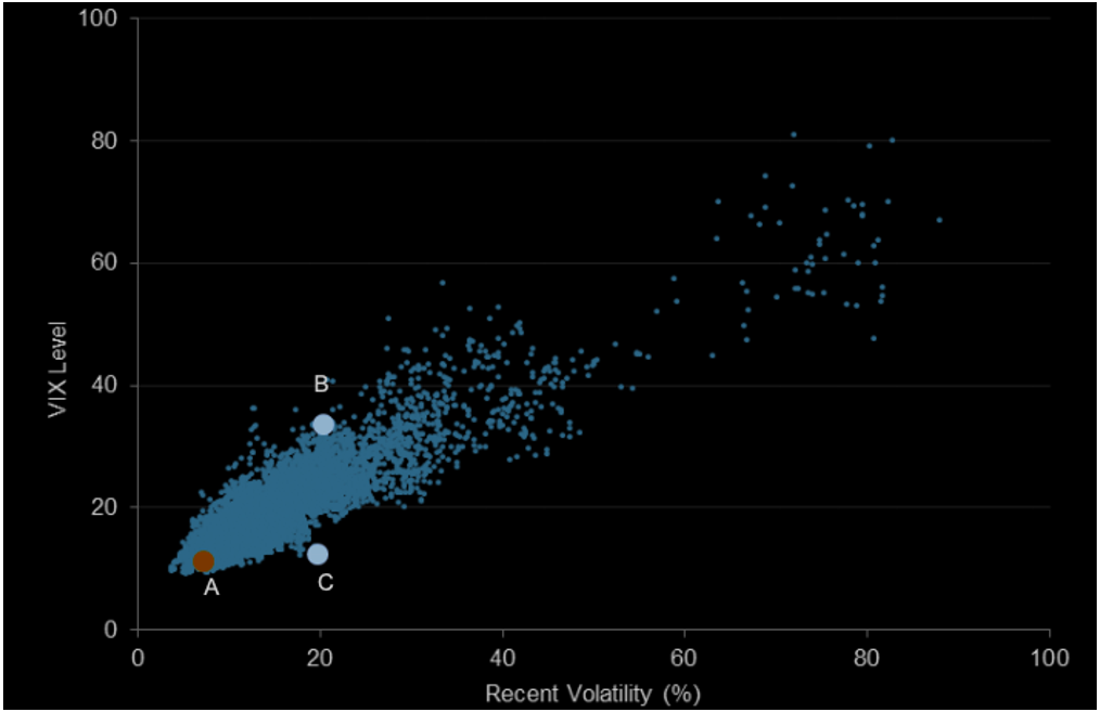
Figure 3 demonstrates that the VIX index is strongly correlated with recent market volatility. However, there is considerable variance; for example, a recent volatility level of about 20% has been associated with a VIX level of 34 (point B, when VIX was very “high”) and with a VIX level of 12 (point C, when VIX was relatively “low”). Volatility (realized or implied) has a strong propensity to return to its mean. This insight is not especially original, despite its illustrious past. There is an enormous body of data demonstrating that volatility tends to mean revert across markets, and the pioneers of this field were given the Nobel Prize in part for incorporating their results into volatility forecasts and simulations (S&P Global Research, 2017).

Figure 3. Relation between VIX and recent volatility.

Source: S&P Global Research (2017).

Realized volatility in the S&P500 index and VIX level

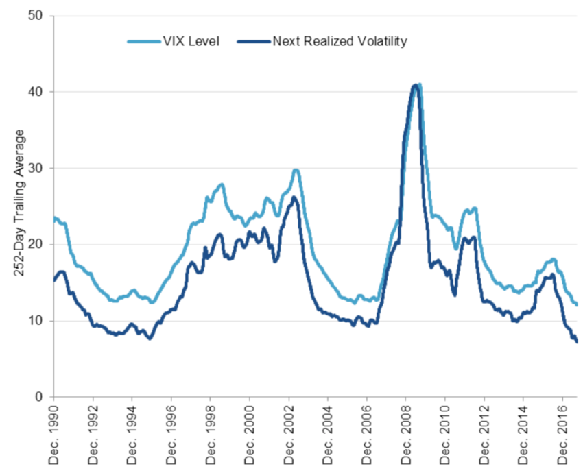
Figure 4 represents the relationship between Realized volatility in the S&P500 index over a period and the VIX level at the begining of the period.

Figure 4. VIX versus next realized volatility.

Source: S&P Global Research (2017).

Mean reversion

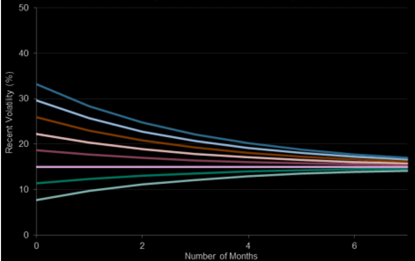
Figure 5 shows how VIX index converge to a certain llong-term level as time passes. This finding is not due to 15% being exceptional in any manner; this figure for M was calculated using historical volatility levels for the S&P 500 and their evolution. It is not implausible that M (else referred to as long-term average volatility in the US equities market) may change over time; changes in the S&P 500’s sector weightings, trade All of these factors have the ability to influence both the pace and the volume and the point at which mean reversion occurs.

Figure 5. Mean-reversion dynamic in recent volatility.

Source: S&P Global Research (2017).

Use of the VIX index in financial markets

There are two methods for determining an asset’s volatility. Either through a statistical calculation of an asset’s realized volatility, also known as historical volatility, which serves as a pointer to the asset’s volatility behavior. This is a limited method that is based on the premise that past volatility tends to replicate itself in the future, without including a forward-looking study of volatility. The second technique is to extract an asset’s volatility from option prices referred to as “implied volatility”.

Why should I be interested in this post?

When investors make investment decisions, they utilize the VIX to gauge the degree of risk, worry, or stress in the market. Additionally, traders can trade the VIX using a range of options and exchange-traded products, or price derivatives using VIX values.

Useful resources

Business analysis

CBOE , 2021. VIX

Nasdaq, 2021. Realized Volatility

Nasdaq, 2021. Vix Index Volatility

S&P Global Research, 2017. Reading VIX: Does VIX Predict Future Volatility?

S&P Global Research, 2017. A Practitioner’s Guide to Reading VIX

About the author

The article was written in September 2021 by Youssef LOURAOUI (ESSEC Business School, Global Bachelor of Business Administration, 2017-2021).

Brownian Motion in Finance

January 30, 2024September 6, 2021 by Jayati WALIA

Brownian Motion in Finance

In this article, Jayati WALIA (ESSEC Business School, Grande Ecole Program – Master in Management, 2019-2022) explains the Brownian motion and its applications in finance to model asset prices like stocks traded in financial markets.

Introduction

Stock price movements form a random pattern. The prices fluctuate everyday resulting from market forces like supply and demand, company valuation and earnings, and economic factors like inflation, liquidity, demographics of country and investors, political developments, etc. Market participants try to anticipate stock prices using all these factors and contribute to make price movements random by their trading activities as the financial and economics worlds are constantly changing.

What is a Brownian Motion?

The Brownian motion was first introduced by botanist Robert Brown who observed the random movement of pollen particles due to water molecules under a microscope. It was in the 1900s that the French mathematician Louis Bachelier applied the concept of Brownian motion to asset price behavior for the first time, and this led to Brownian motion becoming one of the most important fundamental of modern quantitative finance. In Bachelier’s theory, price fluctuations observed over a small time period are independent of the current price along with historical behavior of price movements. Combining his assumptions with the Central Limit Theorem, he also deduces that the random behavior of prices can be said to be represented by a normal distribution (Gaussian distribution).

This led to the development of the Random Walk Hypothesis or Random Walk Theory, as it is known today in modern finance. A random walk is a statistical phenomenon wherein stock prices move randomly.

When the time step of a random walk is made infinitesimally small, the random walk becomes a Brownian motion.

Standard Brownian Motion

In context of financial stochastic processes, the Brownian motion is also described as the Wiener Process that is a continuous stochastic process with normally distributed increments. Using the Wiener process notation, an asset price model in continuous time can be expressed as:

brownian motion equation

with dS being the change in asset price in continuous time dt. dX is the random variable from the normal distribution (N(0, 1) or Wiener process). σ is assumed to be constant and represents the price volatility considering the unexpected changes that can result from external effects. μdt together represents the deterministic return within the time interval with μ representing the growth rate of asset price or the ‘drift’.

When the market is modeled with a standard Brownian Motion, the probability distribution function of the future price is a normal distribution.

Geometric Brownian Motion

weiner notation

When the market is modeled with a geometric Brownian Motion, the probability distribution function of the future price is a log-normal distribution.

Properties of a Brownian Motion

Continuity: Brownian motion is the continuous time-limit of the discrete time random walk. It thus, has no discontinuities and is non-differential everywhere.
Finite: The time increments are scaled with the square root of the times steps such that the Brownian motion is finite and non-zero always.
Normality: Brownian motion is normally distributed with zero mean and non-zero standard deviation.
Martingale and Markov Property: Martingale property states that the conditional expectation of the future value of a stochastic process depends on the current value, given information about previous events. The Markov property instead focusses on the ‘no memory’ theory that the expected future value of a stochastic process does not depend on any past values except the current value. Brownian motion follows both these properties.

Simulating Random Walks for Stock Prices

In quantitative finance, a random walk can be simulated programmatically through coding languages. This is essential because these simulations can be used to represent potential future prices of assets and securities and work out problems like derivatives pricing and portfolio risk evaluation.

A very popular mathematical technique of doing this is through the Monte Carlo simulations. In option pricing, the Monte Carlo simulation method is used to generate multiple random walks depicting the price movements of the underlying, each with an associated simulated payoff for the option. These payoffs are discounted back to the present value and the average of these discounted values is set as the option price. Similarly, it can be used for pricing other derivatives, but the Monte Carlo simulation method is more commonly used in portfolio and risk management.

For instance, consider Microsoft stock that has a current price of $258.65 with a growth trend of 55.2% and a volatility of 35.92%.

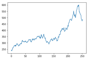
A plot of daily returns represented as a random normal distribution is:

Normal Distribution

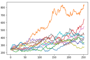
The above figure represents the simulated price path according to the Geometric Brownian motion for the Microsoft stock price. Similarly, a plot of 10 such simulations would be like this:

Microsoft GBM Simulations

Thus, we can see that with just 10 simulations, the prices range from $100 to over $600. We can increase the number of simulations to expand the data set for analysis and use the results for derivatives pricing and many other financial applications.

Brownian motion and the efficient market hypothesis

If the market is efficient in the weak sense (as introduced by Fama (1970)), the current price incorporates all information contained in past prices and the best forecast of the future price is the current price. This is the case when the market price is modelled by a Brownian motion.

▶ Jayati WALIA Black-Scholes-Merton option pricing model

▶ Jayati WALIA Plain Vanilla Options

▶ Jayati WALIA Derivatives Market

Useful Resources

Academic articles

Fama E. (1970) Efficient Capital Markets: A Review of Theory and Empirical Work, Journal of Finance, 25, 383-417.

Fama E. (1991) Efficient Capital Markets: II Journal of Finance, 46, 1575-617.

Books

Malkiel B.G. (2020) A Random Walk Down Wall Street: The Time-tested Strategy for Successful Investing, WW Norton & Co.

Code

Python code for graphs and simulations

Brownian Motion

What is the random walk theory?

About the author

The article was written in August 2021 by Jayati WALIA (ESSEC Business School, Grande Ecole Program – Master in Management, 2019-2022).

Introduction

The Black-Scholes-Merton model

Key Parameters

Option payoff

Call option value

Option and volatility

Volatility: the unobservable parameter of the model

Implied Volatility

Calculating Implied volatility

Newton-Raphson Method

Why should I be interested in this post?

Related posts on the SimTrade blog

Useful resources

Academic research

About the BSM model

Other

About the author

Introduction

Practical Example: Analysis of the S&P 500 Index

Prices

Returns

Distribution of returns

Standard deviation of the distribution of returns

Annualized volatility

Annualized mean

Application: Estimating the Future Price Range of the S&P 500 index

Historical Volatility

Unconditional Volatility

Rolling historical volatility

Alterative measures of volatility

Parkinson volatility

Implied volatility

ARCH model

Stochastic volatility models

Applications in finance

The normal distribution

Brownian motion

Modern Portfolio Theory (MPT)

Capital Asset Pricing Model (CAPM)

Why should I be interested in this post?

Related posts on the SimTrade blog

Risk and Volatility

Portfolio Theory and Models

Financial Indexes

Useful Resources

Academic research

Other

About the author

Introduction

Weather Risk and Agricultural Markets

Case Study: Weather Shocks in Wheat Markets

Climate-Based Volatility in Derivatives Pricing

Why should I be interested in this post?

Related posts on the SimTrade blog

Useful resources

About the author

Introduction

Computation methods for implied volatility

Example

Volatility smile

Volatility surface

CBOE Volatility Index

Related posts on the SimTrade blog

Useful resources

Academic articles

Business

About the author

Definition

Mathematical formulae

Measure of volatility

Example: Apple Stock

Related posts on the SimTrade blog

Useful resources

About the author

VIX index

Definition

Behavior of the VIX index

Statistical distribution of the S&P500 index returns and VIX level

Recent volatility in the S&P500 index and VIX level

Realized volatility in the S&P500 index and VIX level