VIX Futures and Options

Saral BINDAL

In this article, Saral BINDAL (Indian Institute of Technology Kharagpur, Metallurgical and Materials Engineering, 2024–2028; Research Assistant at ESSEC Business School) examines the characteristics, pricing, and settlement of VIX futures and options, along with their term structure and market microstructure.

Introduction

The Cboe Volatility Index (VIX) is a real-time measure of the market’s expectation of S&P 500 volatility over the next 30 days. It is calculated from the prices of S&P 500 Index (SPX) options and is expressed as an annualized percentage. The VIX is widely used as a measure of expected market volatility. For more details, see the previous posts on Implied Volatility and Option Prices and Cboe Volatility Index.

The VIX itself is an index and cannot be directly bought or sold. To allow market participants to trade volatility, Cboe introduced VIX derivatives such as futures and options. VIX futures were introduced in 2004, followed by VIX options in 2006. VIX futures provide linear exposure to changes in the market’s pricing of the future level of the VIX Index, while VIX options provide nonlinear exposure, allowing investors to take positions on changes in the VIX through a range of strike prices and maturities.

VIX Futures

A VIX futures contract is a standardized agreement whose value is linked to the VIX Index at a specified future date (expiration date of the contract). A VIX futures contract reflects the market’s pricing of the VIX Index at a specified future expiration date. Its price incorporates expectations about future volatility as well as risk premia and therefore should not necessarily be interpreted as an unbiased forecast of the future VIX level. VIX futures are traded on the Cboe Futures Exchange (CFE) under the symbol VX.

The pricing of VIX futures differs from that of conventional futures on a tradable stock or stock index. For a stock, the futures price can be related to the current spot price through a cash-and-carry arbitrage relationship, typically expressed as F0 = S0e(r-q)T, where r is the interest rate and q is the dividend yield. This relationship relies on the ability to buy and hold the underlying asset. In contrast, the VIX is an index and cannot itself be directly bought or held. Therefore, the VIX futures contract does not simply represent the current VIX value carried forward to a future date. Instead, it is a market price determined by participants’ expectations about future volatility (the expected value of VIX at maturity), together with the supply and demand for volatility exposure and the risk associated with holding the contract.

VIX futures have a $1,000 contract multiplier. Therefore, a one-point change in the price of a VIX futures contract corresponds to a $1,000 change in the value of one contract.

For example, if an investor buys one VIX futures contract at 20 and its price subsequently rises to 23, the change of 3 VIX points corresponds to a gain of:

VIX Futures Calculation Example

before transaction costs and any financing or opportunity costs associated with margin requirements.

Transaction Costs

Trading VIX derivatives involves both explicit (commissions and fees) and implicit (price impact) transaction costs. These affect the cost of entering and exiting positions and, ultimately, strategy performance. These costs can be broken down into the following components:

Brokerage commissions: Fees charged by brokers for executing trades.

Exchange transaction fees: Fees levied by the exchange on executed contracts.

Clearing and regulatory fees: Charges associated with clearing trades and applicable regulatory requirements.

Bid-ask spread: The difference between the best available ask and bid prices. Crossing the spread creates an immediate execution cost, which varies with market liquidity and volatility.

Slippage: The difference between the expected and actual execution prices. It can arise from market movements, order size and limited liquidity, particularly during periods of elevated volatility.

Margin Requirements and Costs

Unlike transaction costs, margin is not a fee paid to execute a trade. It is the collateral required to maintain a derivatives position, tying up capital that could otherwise be deployed elsewhere.

When opening a position, a trader must meet the initial margin requirement. As the position is marked to market, gains and losses affect the account balance. If losses reduce the balance below the maintenance margin requirement, additional funds may be needed to keep the position open.

The cost of margin therefore lies primarily in the capital committed to the trade and its associated opportunity cost. Traders may also incur financing costs if they borrow funds to meet margin requirements. These considerations become particularly important in VIX derivatives, where margin requirements can change with market conditions and increase during periods of elevated volatility.

Settlement of VIX Futures

VIX futures are cash-settled. Unlike futures on physical commodities, there is no delivery of an underlying asset at expiration because the VIX itself is an index and not a traded asset. Instead, the final profit or loss is determined using the final settlement value of the contract.

The final settlement value is determined on the morning of the expiration date, usually a Wednesday, through a Special Opening Quotation (SOQ) of the VIX Index. The SOQ is calculated using the VIX methodology applied to the relevant SPX options and determines the final settlement value of the VIX futures contract. As expiration approaches, the futures price converges toward this settlement value, reflecting the contract’s approaching expiration.

For a long VIX futures position, the profit or loss at settlement can be represented as:

VIX Futures Payoff Formula

For example, suppose an investor purchases one VX futures contract at 20. If the final settlement value is 28, the investor receives:

VIX Futures Calculation Example 2

Thus, the cash-settlement mechanism allows investors to gain or lose based on changes in the market’s pricing of volatility without owning the underlying SPX options used in the VIX calculation.

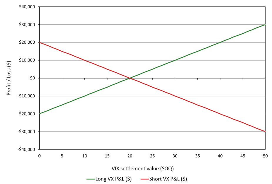
Figure 1 below illustrates the VIX Futures P&L at Settlement for both long and short positions as a function of the VIX value at maturity, for a VX futures contract bought (long) or sold (short) at a futures price of 20. The contract has a multiplier of $1,000 per index point and is cash-settled at maturity at the Special Opening Quotation (SOQ) of the VIX Index.

Figure 1. VIX Futures P&L at Settlement
VIX Futures P&L at Settlement
Source: computation by the author.

VIX Futures Term Structure

A term structure exists because VIX futures contracts have different expiration dates and therefore reflect market expectations over different future periods. As the time to expiration changes, the information, uncertainty, and expected volatility associated with that future period also change, causing futures contracts with different maturities to trade at different prices.

An upward-sloping term structure indicates that VIX futures with later expiration dates are priced at higher VIX levels than contracts with nearer expirations. This is known as contango. By contrast, a downward-sloping term structure indicates that VIX futures with later expiration dates are priced at lower VIX levels than contracts with nearer expirations. This is known as backwardation.

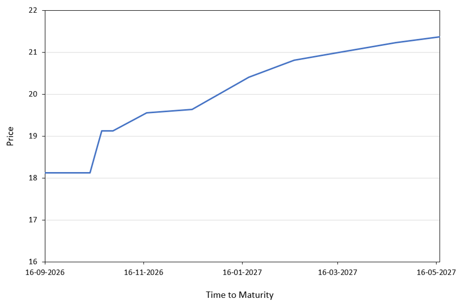
Figure 2 below illustrates the VIX Futures Term Structure using data obtained from Cboe, covering expiration dates from September 16, 2026, to May 18, 2027. The figure shows an upward-sloping curve, indicating a state of contango. This suggests that VIX futures contracts with later expiration dates are priced at higher levels than those with nearer expirations, indicating that the market assigns higher prices to longer-dated volatility exposure.

Figure 2. VIX Futures Term Structure (September 2026)
VIX Futures Term Structure
Source: computation by the author (Cboe data).

This term structure has implications for investors who maintain long positions in VIX futures. As contracts approach expiration, investors seeking to maintain their exposure must sell the expiring contracts and buy later-dated ones. In a contango market, longer-dated futures contracts trade at higher prices than nearer-dated contracts. Maintaining a long futures exposure therefore involves replacing expiring contracts with higher-priced contracts. Although contango can create a negative roll effect for long futures strategies, the realized return depends on subsequent changes in futures prices and the specific rolling strategy. For long positions, this can create a drag on returns as futures prices evolve toward settlement. However, the outcome depends on how futures prices change over time, rather than on contango alone. The relationship between trading demand, futures pricing and the term structure is discussed further in the market microstructure section below.

VIX Options

VIX options are exchange-traded derivatives that provide nonlinear exposure to the VIX settlement value at expiration. Their pricing is closely related to the corresponding VIX futures contract rather than solely to the current spot level of the VIX Index. VIX options are traded on Cboe Options Exchange and are based on the Cboe Volatility Index (VIX). Unlike individual stocks in stock options, the VIX is itself an index derived from prices of S&P 500 Index (SPX) options.

Cboe offers both monthly and weekly VIX option expirations, providing market participants with different maturities for expressing views on volatility.

Each VIX option contract has a $100 multiplier. Therefore, the dollar value of an option is obtained by multiplying its quoted premium by $100.

For example, if an investor buys one VIX call option with a strike price of 20 and the VIX settlement value is 15 at expiration, the option finishes 5 VIX points out-of-the-money. Consequently, the option expires worthless, with a payoff of zero (before accounting for the premium paid, transaction costs, and other applicable charges).

Settlement of VIX Options

VIX options are cash-settled. This means that there is no physical delivery of an underlying asset when an option is exercised. Instead, the value of an exercised option is determined using the final settlement value of the VIX.

The final settlement value is determined on the morning of the expiration date, usually a Wednesday through a Special Opening Quotation (SOQ) of the VIX Index. The SOQ is calculated using the VIX methodology applied to the relevant SPX options and is used to determine the final settlement value of the VIX option.

For a VIX call option, the settlement value is based on the amount by which the final VIX settlement value exceeds the strike price, and for a VIX put option, the settlement value is based on the amount by which the strike price exceeds the final VIX settlement value.

For a call option, this can be represented as:

VIX Call Option Payoff Formula

For a put option:

VIX Put Option Payoff Formula

For example, suppose an investor holds a VIX call option with a strike price of 20 and the final settlement value is 28. The option’s settlement value is:

VIX Options Calculation Example 2

If the final settlement value is below 20, the call expires without value.

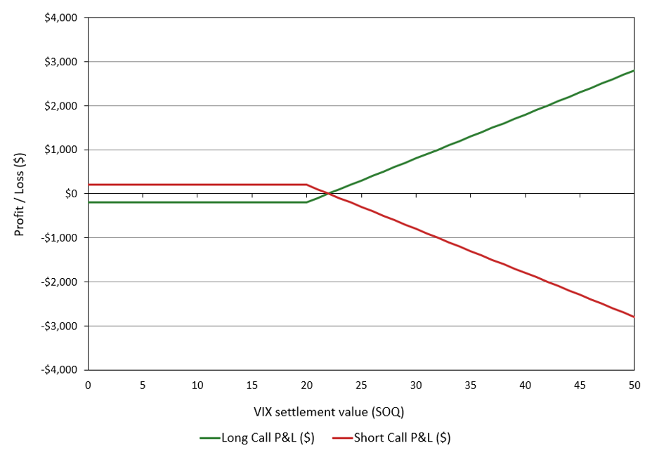
Figure 3 illustrates the P&L at expiration for long and short VIX call positions as a function of the VIX value at maturity. For a strike price of 20, a premium of 2.00 VIX points, and a $100 multiplier, the long call has a maximum loss of $200 when the VIX settles at or below 20 and unlimited gain above the breakeven level of 22. VIX options are cash-settled at expiration based on the VIX SOQ.

Figure 3. VIX Call Option P&L at Settlement
VIX Call Option P&L at Settlement
Source: computation by the author.

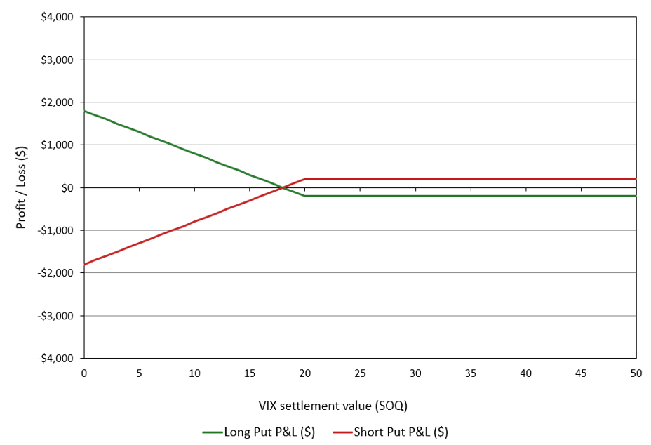
Figure 4 illustrates the P&L at expiration for long and short VIX put positions as a function of the VIX value at maturity. For a strike price of 20, a premium of 2.00 VIX points, and a $100 multiplier, the long put has a maximum loss of $200 when the VIX settles at or above 20 and becomes profitable below the breakeven level of 18. VIX options are cash-settled at expiration based on the VIX SOQ.

Figure 4. VIX Put Option P&L at Settlement
VIX Put Option P&L at Settlement
Source: computation by the author.

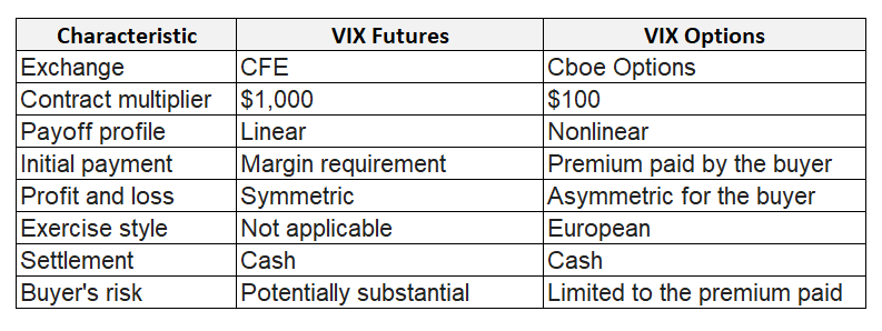
The table below summarizes the key characteristics of VIX futures and options contracts discussed above.

Figure 5. Key Characteristics of VIX Futures and VIX Options
 Key Characteristics of VIX Futures and VIX Options
Source: computation by the author.

Market Participants

VIX futures and options involve several types of market participants with different objectives.

Institutional investors and asset managers may use VIX derivatives to hedge portfolios against changes in market volatility.

Hedge funds and proprietary trading firms may use VIX futures and options to speculate on future movements in volatility or implement volatility-related strategies.

Market makers provide liquidity by quoting prices at which they are willing to buy and sell VIX derivatives, facilitating trading in these instruments.

Individual investors can also access VIX futures and options through eligible brokers, subject to account approval, margin requirements and regional availability. They may use these instruments to speculate on changes in expected market volatility or to hedge equity-market exposure. However, access to these products does not imply that they are suitable for all investors, given their leverage, complexity and potential for substantial losses.

Other market participants may combine VIX futures, VIX options, SPX options, and other volatility-related instruments to construct different trading and hedging strategies.

Market Microstructure

Prices in financial markets emerge from the interaction between buyers and sellers. In the conventional microeconomic framework, the demand curve represents the quantities buyers are willing to purchase at different prices, while the supply curve represents the quantities sellers are willing to offer. Their intersection determines the market equilibrium, where quantity demanded equals quantity supplied. In practice, trading mechanisms can take different forms like an electronic order book or block trading arrangements for large transactions. Demand and supply are influenced by market participants’ expectations of future prices (volatility for VIX futures and option markets).

VIX futures and options are traded on electronic markets where buyers and sellers submit orders. Market participants can use different order types, particularly market orders and limit orders. In the VIX futures market, limit orders are recorded in an electronic order book, which displays outstanding buy and sell orders along with their prices and quantities. Incoming orders are matched against existing orders according to the exchange’s matching rules. The highest price buyers are willing to pay is the best bid, while the lowest price sellers are willing to accept is the best ask. The difference between these two prices is the bid-ask spread, which represents an important component of transaction costs. Market depth refers to the quantities available for trading at different price levels. Together, the bid-ask spread and market depth provide useful indicators of market liquidity and the potential price impact of executing an order.

VIX options also trade electronically. Market makers provide quotes and may supply liquidity by taking the opposite side of a trade. Multi-leg strategies, such as vertical spreads, present an additional execution challenge because the trader needs to buy and sell options at a suitable combined price. Cboe’s Complex Order Book (COB) allows these orders to be matched as a combined position, while its Complex Order Auction (COA) gives eligible orders an opportunity for price improvement.

For large VIX futures positions, block trades offer an alternative to execution through the displayed order book. Eligible counterparties can negotiate a transaction privately and report it to the exchange under the applicable rules. This can help participants execute large orders without relying entirely on the liquidity available in the electronic market.

Trading prices also differ from the value used to settle contracts at expiration. VIX futures and options are cash-settled using the Special Opening Quotation (SOQ) of the VIX Index on the final settlement date. Unlike the regular VIX calculation, which uses bid-ask midpoints from SPX options across two expirations, the SOQ uses opening trade prices from a single SPX option expiration selected to provide the required 30-day measure. If a selected option has no opening trade price, its bid-ask midpoint is used instead. The resulting SOQ determines the final settlement value of the expiring derivatives.

Price Formation in VIX Futures

A VIX futures price reflects the price at which market participants are willing to trade exposure to the VIX Index at a specified future expiration. It is not necessarily an unbiased forecast of the VIX level at that date. The VIX measures expected 30-day volatility derived from S&P 500 index options, whereas a VIX futures contract provides exposure to the value of this index at its own expiration. Futures prices therefore reflect expectations about future volatility conditions, risk premia and the balance of buying and selling pressure.

The relationship between futures prices across expiration dates is described by the VIX futures term structure. In contango, longer-dated contracts trade above nearer-dated contracts; in backwardation, nearer-dated contracts trade above longer-dated ones. Contango is frequently observed in relatively calm markets, while backwardation can emerge during periods of market stress, when demand for near-term volatility exposure increases sharply. However, an upward-sloping futures curve does not necessarily imply that the market expects the spot VIX to rise. The curve also reflects risk premia and supply and demand for volatility exposure across different maturities.

Trading activity can influence both the overall level of futures prices and the relative pricing of contracts with different expiration dates. Mixon and Onur (2019) examine how non-dealer trading activity relates to VIX futures pricing. Their findings highlight the role of aggregate net demand in the overall level of futures prices and the relationship between trading activity in individual contracts and the shape of the futures curve. This is relevant to the roll effect, which describes the contribution to returns from replacing a futures contract approaching expiration with a later-dated contract. In contango, maintaining a long position typically involves selling a nearer-dated contract and buying a more expensive deferred contract. This can create a headwind for returns, although the realised outcome depends on subsequent futures-price movements and the investor’s rolling strategy.

Price Formation in VIX Options

The price of a VIX option depends on the possible VIX settlement values at expiration relative to the option’s strike price. A call option has a positive payoff when the final settlement value exceeds the strike, while a put option has a positive payoff when the settlement value falls below the strike. The option premium reflects the potential payoffs, the time remaining until expiration, interest rates and the market’s assessment of the distribution of possible settlement values.

VIX futures play an important role in standard VIX option valuation. Because the VIX Index itself is not directly tradable, VIX futures provide market-based information about volatility priced for specific future dates. The relevant futures price is an important input in option valuation, but it does not determine the option premium on its own. The strike price, time to expiration, interest rates and the distribution of possible settlement values also influence the premium.

Option prices vary across strike prices and expiration dates. Implied volatility, calculated from observed option premiums using an option-pricing model, provides a common measure for comparing these prices. The implied volatility skew describes variation in implied volatility across strike prices, while the term structure describes variation across option maturities. These patterns show how the market prices options with different payoff profiles and maturities.

Tong, Huang and Wang (2022) compare VIX option pricing models that use the VIX Index and VIX futures as state variables, meaning market variables used as model inputs. Their findings indicate that models incorporating VIX futures prices perform better empirically than models relying on the VIX Index alone and several alternative market variables. This highlights the importance of futures-market information in modelling and valuing standard VIX options.

Trading Activity and Market Liquidity

In this section, we examine the trading activity and relative scale of the S&P 500 and VIX derivatives markets by comparing the average daily volumes of their futures and options contracts. The data are sourced from CME Group and Cboe.

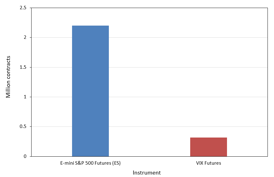
Figure 6 below compares the average daily trading volume of E-mini S&P 500 futures and VIX futures in March 2026. E-mini S&P 500 futures (ES) are standardized futures contracts on the S&P 500 Index, with a contract multiplier of $50 per index point. ES recorded an average daily volume of 2.2 million contracts (CME Group), compared with 0.318 million contracts for VIX futures (Cboe).

Figure 6. Average daily number of contracts of S&P 500 and VIX futures (March 2026)
Average Daily Number of Contracts of S&P 500 and VIX Futures, March 2026
Source: computation by the author (CME Group and Cboe data).

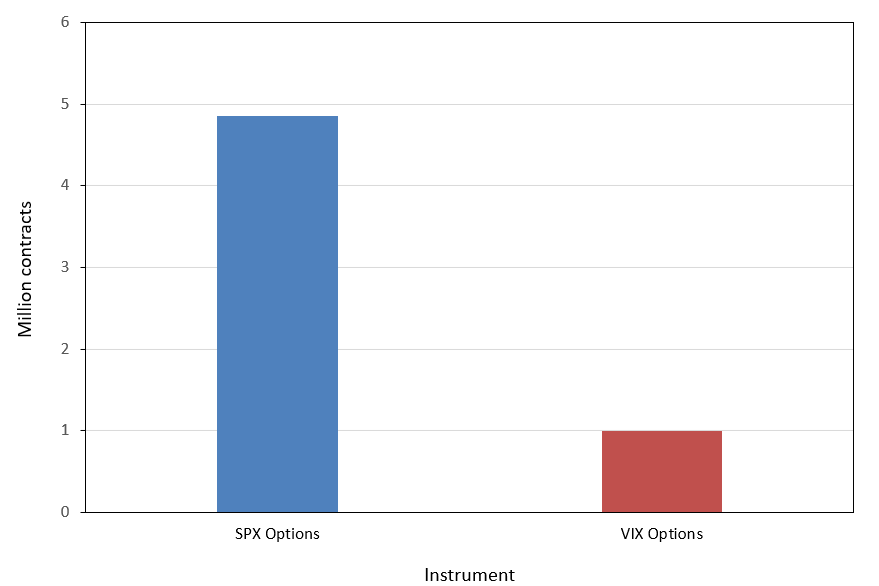
Figure 7 below compares the average daily number of contracts (a proxy for trading activity) of S&P 500 Index (SPX) options and VIX options during Q1 2026. SPX options recorded an average daily volume of 4.855 million contracts (Cboe), while VIX options recorded 0.994 million contracts (Cboe). The figures represent average daily volume across January, February, and March 2026.

Figure 7. Average daily number of contracts of S&P 500 and VIX options (Q1 2026)
Average Daily Number of Contracts of S&P 500 and VIX Options (Q1 2026)
Source: computation by the author (Cboe data).

The figures provide an indication of the relative trading activity in S&P 500 and VIX derivatives, but they should be interpreted with caution. Average daily trading volume, measured in contracts, differs from the monetary or notional value of transactions. A higher contract volume does not necessarily imply a proportionally larger market in terms of economic exposure or liquidity. Furthermore, trading volume alone does not fully capture liquidity, which also depends on bid-ask spreads, market depth (number of contracts available in the market at a given price), and execution costs (bid-ask spreads, commissions, and the price impact of a trade). Therefore, the figures are best interpreted as a comparison of trading activity rather than a direct measure of market size or relative liquidity.

Why should I be interested in this post?

VIX futures and options are important instruments for market participants to take positions on future volatility, hedge portfolios against changes in volatility, and manage exposure to market risk. Understanding these instruments therefore provides a practical perspective on the management of volatility risk in financial markets.

Related posts on the SimTrade blog

Futures

   ▶ Akshit GUPTA Futures Contract

   ▶ Alexandre VERLET Understanding financial derivatives: futures

Options

   ▶ Akshit GUPTA Options

   ▶ Jayati WALIA Black-Scholes-Merton Option Pricing Model

   ▶ Jayati WALIA Implied Volatility

   ▶ Saral BINDAL Implied Volatility and Option Prices

VIX

   ▶ Youssef LOURAOUI VIX index

   ▶ Saral BINDAL Cboe Volatility Index

   ▶ Saral BINDAL VIX Data and Statistical Properties

Useful resources

Business resources

CME Group (2026) March 2026 Trading Volume.

Cboe Global Markets (2026) March 2026 Monthly Volume Statistics.

Cboe Global Markets (2026) VIX Futures.

Cboe Global Markets (2026) VIX Options.

Academic references

Black F. (1976) The pricing of commodity contracts, Journal of Financial Economics, 3, 167-179.

Carr P. and L. Wu (2006) A tale of two indices. The Journal of Derivatives, 13(3), 13-29.

Mixon S. and Onur E. (2019) Derivatives Pricing When Supply and Demand Matter: Evidence from the Term Structure of VIX Futures. The Journal of Futures Markets, 39(9), 1035-1055.

Tong C., Huang Z. and Wang T. (2022) Do VIX Futures Contribute to the Valuation of VIX Options? The Journal of Futures Markets, 42(9), 1644-1664.

Whaley R. E. (2009) Understanding the VIX. The Journal of Portfolio Management, 35(3), 98-105.

Zhang J. E. and Y. Zhu (2006) VIX futures. Journal of Futures Markets, 26(6), 521-531.

About the author

The article was written in October 2026 by Saral BINDAL (Indian Institute of Technology Kharagpur, Metallurgical and Materials Engineering, 2024-2028 & Research assistant at ESSEC Business School). His interests include tracking geopolitical developments and analyzing their direct impact on macroeconomic factors such as inflation, trade balances, and currency volatility, with a focus on using data to quantify these global economic ripple effects.

Discover all posts by Saral BINDAL
VIX Data and Statistical Properties

Saral BINDAL

In this article, Saral BINDAL (Indian Institute of Technology Kharagpur, Metallurgical and Materials Engineering, 2024-2028 & Research assistant at ESSEC Business School) examines the statistical properties of historical VIX data and applies statistical methods to model its dynamics.

Introduction

The Chicago Board Options Exchange (CBOE) Volatility Index, or VIX, is a real-time market index designed to measure the market’s expectation of 30-day forward-looking annualized volatility in the US equity market. It is option-based, calculated using the market prices of S&P 500 index options to gauge expected volatility. The VIX construction methodology can be found in the article CBOE Volatility Index

In this article, we analyze the VIX index using historical market data to study its statistical properties, and discuss the methods used to model its dynamics in quantitative finance.

Historical Data

The VIX Index Historical data is publicly available from the Chicago Board Options Exchange (CBOE) and is updated on a daily basis. The analysis in this article is based on daily closing values of the VIX obtained from this data.

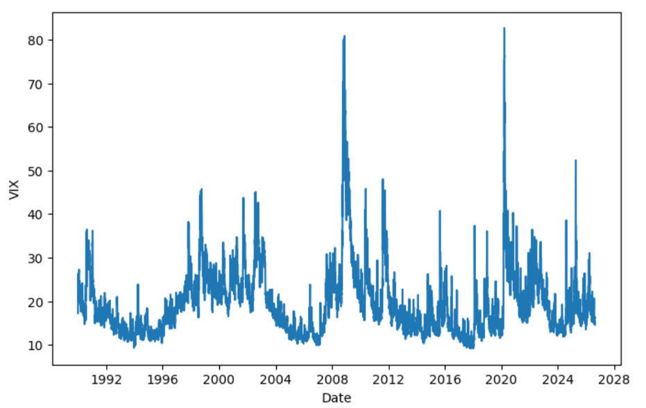
Figure 1 below illustrates the time series plot of VIX daily closing values from January 1990 to August 2026. From the figure, we can observe that during periods of high uncertainty, the VIX tends to rise significantly, as seen during the Global Financial Crisis (2007–2009) and the COVID-19 pandemic (2019–2020). We can also see the VIX rising as of now amid the ongoing Middle East crisis, although not to the same extent as observed during previous periods of heightened uncertainty.

Figure 1. VIX Index Historical Data (1990-2026)
VIX Index Historical Data (1990-2026)
Source: computation by the author.

Distributional Characteristics

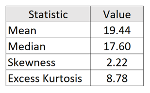
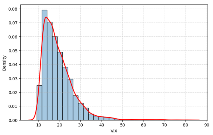
Using historical VIX data from 1990 to 2026, Figure 2 illustrates the empirical distribution of daily VIX closing values. The histogram, overlaid with a kernel density estimate (KDE), provides a visual representation of the distribution’s underlying probability density. The corresponding first four moments of the distribution are reported below:

Table 1. VIX Distribution Statistics
Table of VIX Distribution Statistics
Source: computation by the author.

From the above table, we can observe that the data is right-skewed, which indicates that volatility tends to remain relatively low under normal market conditions but can rise sharply during periods of financial stress. The long right tail therefore reflects the occurrence of volatility shocks and tail-risk events, such as the Global Financial Crisis (2007–2009), the COVID-19 market shock (2020), and other episodes of significant financial or geopolitical uncertainty. Moreover, a high excess kurtosis indicates fatter tails compared to a normal distribution, implying a higher probability of observing extreme VIX levels. From the histogram, we observe that the VIX is concentrated around a level of 15 for a large proportion of the sample. This suggests that, under normal market conditions, the VIX tends to fluctuate around this level, which can be interpreted as its long-term level of the market uncertainty

Figure 2. Historical Distribution and Kernel Density Estimation of the Daily VIX levels
Historical Distribution of the Daily VIX levels
Source: computation by the author.

Time-Series Properties

The VIX exhibits several well-documented time-series properties that distinguish it from traditional financial asset prices. Unlike equity prices, whose levels are generally characterized by non-stationary dynamics, the VIX exhibits pronounced mean reversion and persistence, together with sharp spikes during episodes of market stress. The mean-reverting behaviour of the VIX is particularly noteworthy because it resembles a fundamental feature of interest-rate dynamics, which has long been incorporated into models such as the Vasicek (1977) and Cox, Ingersoll, and Ross (1985). The mean-reverting specifications have similarly been used to capture the tendency of volatility to return toward a long-run level.

However, the two processes differ substantially in their temporal dynamics. Interest-rate persistence typically reflects gradual adjustments in response to macroeconomic conditions and monetary policy, with mean reversion occurring over relatively longer horizons. In contrast, the VIX responds rapidly to changes in market expectations: episodes of financial stress can trigger abrupt upward spikes, followed by relatively rapid mean reversion toward lower levels. Thus, while both exhibit persistent and mean-reverting dynamics, the VIX is distinguished by its faster adjustment, pronounced asymmetry, and sharp responses to market stress.

Methods to Model VIX Dynamics

VIX dynamics exhibit several distinctive characteristics, particularly mean reversion and persistence, which require different modelling approaches. This section examines how various econometric models capture these features, ranging from mean-reverting and Log-VIX models to HAR, ARCH/GARCH, and stochastic volatility models.

Mean-Reverting Models

Early approaches to modelling volatility indices treated volatility as a mean-reverting stochastic process. A commonly used specification is the Cox-Ingersoll-Ross (CIR) process, originally developed for interest-rate modelling by Cox, Ingersoll and Ross (1985) and subsequently applied to volatility derivatives by Grünbichler and Longstaff (1996). Grünbichler and Longstaff modelled the volatility index using a mean-reverting square-root process and derived pricing formulas for volatility futures and options.

The dynamics are given by


CIR Formula

  • Vt represents the volatility index at time t
  • κ is the speed of mean reversion
  • θ is the long-run level towards which the process tends to revert
  • σ is the diffusion parameter controlling the magnitude of random fluctuations
  • Wt is a standard Brownian motion

The term κ(θ − Vt)dt represents the mean-reverting component, which pulls the process towards its long-run level θ, while σ√VtdWt represents the diffusion component, capturing random fluctuations in the volatility index.

The CIR framework was subsequently examined empirically in the context of VIX futures by Zhang and Zhu (2006). They estimated a stochastic variance model using historical VIX data and used it to derive and evaluate VIX futures prices.

An alternative mean-reverting modelling approach is the Ornstein-Uhlenbeck (OU) process (Uhlenbeck and Ornstein, 1930), which assumes a constant diffusion coefficient:


OU Formula

Unlike the CIR process, the OU process is Gaussian and can theoretically take negative values. This makes the OU process unsuitable for modelling the VIX level directly, since the VIX is strictly positive. A common way to retain the mean-reverting OU structure while ensuring a positive VIX is therefore to model log(VIX) rather than the VIX level itself.

Log-VIX Models

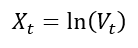
A natural way to address the possibility of negative values is to model the logarithm of the VIX. Let


VIX Log-Change Formula

A mean-reverting logarithmic process can then be written as


Mean Reverting Log Formula

or equivalently,


Mean Reverting Log Formula

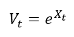
Since


VIX Formula

the resulting modelled VIX is strictly positive. The logarithmic transformation therefore preserves the mean-reverting structure while avoiding the negative-value problem associated with modelling the VIX level using a Gaussian process.

Mean-reverting in the log models were studied by Detemple and Osakwe (2000) in the context of volatility option valuation. Their model provides an early theoretical foundation for modelling volatility through a log-normal mean-reverting process. The approach was subsequently applied directly to the VIX by Bao (2013), who developed a mean-reverting logarithmic model for the spot VIX and extended it to incorporate jumps and stochastic volatility.

Heterogeneous Autoregressive Model

Although continuous-time mean-reverting models capture the tendency of volatility to move towards a long-run level, empirical evidence indicates that the VIX also exhibits substantial persistence across different time horizons. Fernandes, Medeiros and Scharth (2014) conducted a detailed analysis of the time-series properties of the VIX and found evidence of long-range dependence. They therefore employed Heterogeneous Autoregressive (HAR) models to model and forecast the VIX.

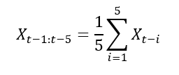
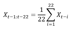
The HAR framework captures persistence by allowing past VIX observations over different horizons to affect the current value. A simplified HAR model can be expressed as


HAR Formula

where


HAR Weekly Component Formula

and


HAR Monthly Component Formula

The three components represent information from daily, weekly, and monthly horizons, respectively. This allows the HAR-VIX model to capture the persistence of the VIX across different time horizons while remaining relatively simple and parsimonious. The HAR framework was originally introduced by Corsi (2009) to model the heterogeneous dynamics of realized volatility. Fernandes, Medeiros and Scharth (2014) adapted this framework to the VIX and showed that its multi-horizon structure provides a useful representation of the strong persistence and long-range dependence in the VIX.

Stochastic Variance of the VIX

The volatility of the VIX itself can vary over time. Rather than assuming that the diffusion coefficient is constant, stochastic-volatility models allow the volatility governing VIX fluctuations to evolve as a separate stochastic process.

Kaeck and Alexander (2013) investigate continuous-time models of VIX dynamics that explicitly incorporate stochastic volatility of volatility. Their analysis considers several one- and two-factor continuous-time models, including affine and non-affine specifications and models with jumps, using VIX data over an extended period.

Conceptually, the model can be represented as


Stochastic Volatility VIX Formula

where

  • VIXt represents the VIX index
  • Vt represents the instantaneous variance governing movements in log-VIX and is itself stochastic
  • κ controls the mean-reversion speed of log-VIX
  • θ represents the long-run level of log-VIX
  • Wt is a Brownian motion driving log-VIX
  • Zt represents the size of a jump in log-VIX
  • Jt is a jump-counting process, with dJt representing the occurrence of jumps


Stochastic Variance Formula

  • κv controls the mean-reversion speed of the variance process
  • θv represents the long-run level of the variance process
  • σv controls the volatility of the variance process, representing the volatility-of-volatility
  • Wtv is a Brownian motion driving the variance process

The key distinction is therefore that the variance of VIX fluctuations is no longer constant. It becomes a state variable that evolves over time.

This additional source of randomness allows the model to capture changes in the intensity of VIX fluctuations and provides a more flexible representation of the sharp and persistent movements observed during periods of financial stress. Kaeck and Alexander’s analysis specifically examines whether stochastic volatility of volatility improves the ability of continuous-time models to describe VIX dynamics.

ARCH and GARCH Models

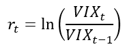
The VIX also exhibits volatility clustering, where periods of high volatility tend to be followed by high volatility, while periods of low volatility tend to be followed by low volatility. This suggests that the variance of log change in VIX is not constant over time. ARCH and GARCH models capture this feature by allowing the conditional variance of log change in VIX to evolve over time.

Let the log change in the VIX be defined as


VIX Log Change Formula

An ARCH or GARCH model can then be used to model the conditional variance of these changes. The standard GARCH(1,1) specification is


GARCH Formula

where

  • rt represents the log change in the VIX at time t
  • μ represents the conditional mean of the VIX log change
  • εt represents the innovation or shock at time t
  • σt2 represents the conditional variance of the VIX log change
  • ω represents the long-run variance component
  • α measures the immediate effect of new shocks on conditional variance
  • β measures the persistence of conditional variance over time

The αεt−12 term captures the immediate impact of a new shock, while the βσt−12 term captures the persistence of previously elevated variance. A high value of β therefore indicates that periods of high variation in the VIX tend to persist.

The ARCH model was introduced by Engle (1982), while Bollerslev (1986) extended it to the more general GARCH framework. For the VIX, these models are useful for studying time-varying conditional variance and volatility clustering in VIX changes, rather than the mean-reverting behaviour of the VIX level itself.

Empirical Analysis of VIX

We use the complete historical daily VIX closing values (1990 – 2026) to estimate the parameters of the CIR model described above. Since the CIR model is specified in continuous time while the data are observed at daily intervals, the process is first discretized using the Euler-Maruyama approximation:


Discretized CIR Formula

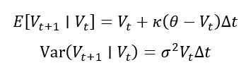
where Δt; = 1/252 for daily observations and εt+1 ∼ N(0,1). This discretization implies that, conditional on the previous day’s VIX value, the expected value and variance of the next observation are:


Conditional Expected Value and Variance Formula

Assuming the discretized process is conditionally normally distributed, these expressions allow us to construct a likelihood for the observed VIX data. The log-likelihood is:


Log Likelihood Formula

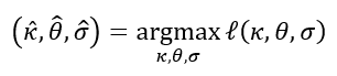
The CIR parameters are then estimated by choosing the values that maximize this log-likelihood:


Maximum Likelihood Estimator Formula

This gives an estimated mean-reversion speed of κ = 4.8618, a long-run VIX level of θ = 19.4237, and a diffusion parameter of σ = 5.1952.

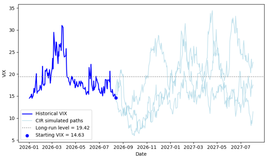
These estimated parameters are then used to simulate a possible future path of the VIX. The simulation starts from the observed VIX value of 14.63 on 13th August 2026 and projects the VIX forward over 252 trading days using the CIR dynamics. The mean-reverting component pulls the process towards the estimated long-run level, while the diffusion component introduces random fluctuations around this tendency.

Figure 3 compares the historical VIX with one simulated path generated by the estimated CIR model. The historical series shows the large fluctuations and sharp spikes observed in the VIX over the sample period, while the simulated path represents one possible future realization starting from the current VIX level of 14.63. The dotted line at 19.42 represents the estimated long-run level of the VIX. The simulated path fluctuates around this level and exhibits a tendency to move towards it, illustrating the mean-reverting behavior implied by the CIR model.

You can download the Excel file with complete historical data used for the above calculations below.

Download the Excel file with complete historical VIX data

Figure 3. Historical Path and Multiple CIR Simulated Paths for the VIX
CIR Simulated Paths
Source: computation by the author.

You can download the Python code below to reproduce the CIR parameter estimation and simulated VIX paths presented above.

Download the Python to simulate the CIR paths.

Alternatively, you can download the R code below with the same functionality as in the Python file.

Download the R code to simulate the CIR paths.

Why should I be interested in this post?

For anyone interested in finance or a career in trading, understanding the statistical properties of VIX and how it is modelled is very important. As one of the most widely used measures of market uncertainty and expected volatility, it serves as an important tool for market analysis, risk assessment and numerous volatility-based trading strategies.

Related posts on the SimTrade blog

   ▶ Akshit GUPTA Options

   ▶ Jayati WALIA Black-Scholes-Merton Option Pricing Model

   ▶ Jayati WALIA Implied Volatility

   ▶ Saral BINDAL Implied Volatility and Option Prices

   ▶ Saral BINDAL Volatility curves: smiles and smirks

   ▶ Youssef LOURAOUI VIX index

Useful resources

Academic research on option pricing

Black F. and M. Scholes (1973) The pricing of options and corporate liabilities. Journal of Political Economy, 81(3), 637-654.

Black, F. (1976), “Studies of Stock Price Volatility Changes”, Proceedings of the Business and Economics Section of the American Statistical Association, 177-181.

Cox J. C., J. E. Ingersoll and S. A. Ross (1985) A theory of the term structure of interest rates. Econometrica, 53(2), 385-407.

Hull J.C. (2022) Options, Futures, and Other Derivatives, 11th Global Edition, Chapter 15 – The Black-Scholes-Merton model, 338-365.

Merton R.C. (1973) Theory of rational option pricing. The Bell Journal of Economics and Management Science, 4(1), 141-183.

Uhlenbeck G. E. and L. S. Ornstein (1930) On the theory of the Brownian motion. Physical Review, 36(5), 823-841.

Academic research on VIX

Bao Q. (2013) Mean-Reverting Logarithmic Modelling of VIX. MPRA Paper, No. 46413.

Bollerslev T. (1986) Generalized autoregressive conditional heteroskedasticity. Journal of Econometrics, 31(3), 307-327.

Corsi F. (2009) A simple approximate long-memory model of realized volatility. Journal of Financial Econometrics, 7(2), 174-196.

Cox J. C., J. E. Ingersoll and S. A. Ross (1985) A theory of the term structure of interest rates. Econometrica, 53(2), 385-407.

Detemple J. and C. Osakwe (2000) The valuation of volatility options. European Finance Review, 4(1), 21-50.

Engle R. F. (1982) Autoregressive conditional heteroscedasticity with estimates of the variance of United Kingdom inflation. Econometrica, 50(4), 987-1007.

Fernandes M., M. C. Medeiros and M. Scharth (2014) Modelling and predicting the CBOE market volatility index. Journal of Banking & Finance, 40, 1-10.

Grünbichler A. and F. A. Longstaff (1996) Valuing futures and options on volatility. Journal of Banking & Finance, 20(6), 985-1001.

Jiang G. J. and Y. S. Tian (2005) The model-free implied volatility and its information content. The Review of Financial Studies, 18(4), 1305-1342.

Kaeck A. and C. Alexander (2013) Continuous-time VIX dynamics: On the role of stochastic volatility of volatility. International Review of Financial Analysis, 28, 46-56.

Uhlenbeck G. E. and L. S. Ornstein (1930) On the theory of the Brownian motion. Physical Review, 36(5), 823-841.

Whaley R. E. (2009) Understanding the VIX. Journal of Portfolio Management, 35(3), 98-105.

Zhang J. E. and Y. Zhu Y. (2006) VIX futures. Journal of Futures Markets, 26(6), 521-531.

VIX Data

CBOE Global Markets (2026) VIX Historical Data.

About the author

The article was written in September 2026 by Saral BINDAL (Indian Institute of Technology Kharagpur, Metallurgical and Materials Engineering, 2024-2028 & Research assistant at ESSEC Business School). His interests include tracking geopolitical developments and analyzing their direct impact on macroeconomic factors such as inflation, trade balances, and currency volatility, with a focus on using data to quantify these global economic ripple effects.

Discover all posts written by Saral BINDAL.

CBOE Volatility Index

Saral BINDAL

In this article, Saral BINDAL (Indian Institute of Technology Kharagpur, Metallurgical and Materials Engineering, 2024-2028 & Research assistant at ESSEC Business School) explains the CBOE methodology for the construction of the volatility index or ‘VIX’.

Introduction

The Chicago Board Options Exchange (CBOE) Volatility Index, or VIX, is a real-time market index designed to measure the market’s expectation of 30-day forward-looking annualized volatility. It is option-based, calculated using the market prices of S&P 500 index options to gauge expected volatility.

History

In 1993, CBOE Global Markets introduced the CBOE Volatility Index (VIX Index). Originally designed by Robert E. Whaley (1993) to measure the market’s expectation of 30-day volatility, the index was calculated using an option-pricing model to derive the implied volatility of at-the-money S&P 100 index (OEX Index) options. The VIX Index quickly became the premier benchmark for U.S. stock market volatility and is widely referred to as the market’s “fear gauge”.

Ten years later in 2003, CBOE partnered with Goldman Sachs to completely overhaul the index. This update introduced a methodology independent of option-pricing models, adapting the seminal theoretical framework for model-free implied variance established by Britten-Jones and Neuberger (2000) alongside the practical replication insights of Demeterfi et al. (1999). This modern version of the VIX shifted its underlying base to the broader S&P 500 index. Rather than tracking a narrow selection of options, it estimates market expectations by aggregating a heavily weighted cross-section of SPX puts and calls across a wide range of strike prices.

Academic research confirms that this model-free aggregation method captures more information and provides a more efficient forecast of future realized volatility than individual Black-Scholes implied volatilities (Jiang & Tian, 2005).

Market Behavior

While VIX is often regarded as the market’s fear index, it might give one a false impression that it moves opposite to the S&P 500. Mathematically it has no directional bias, and only measures the magnitude of expected volatility. Instead, the real-world inverse relationship is driven by corporate capital structures and asymmetric investor behavior. As Black (1976) pointed out, when a stock price drops, a company’s financial leverage automatically increases, making the equity riskier and naturally driving up volatility.

Furthermore, market sell-offs trigger a sudden panic where investors rush to buy portfolio insurance (put options) all at once. Because the supply of this insurance is limited, options market makers must aggressively raise prices to protect themselves. Gârleanu et al. (2009) formalize this mechanism, demonstrating that because market makers cannot perfectly hedge their positions, concentrated investor demand directly drives option pricing and inflates implied volatility premiums. Since the VIX is calculated directly from these option prices, this demand-pressure mechanically forces the index to spike.

This same demand explains why the S&P 500 and the VIX occasionally rise together. During massive market rallies, investors experience FOMO (Fear of Missing Out) and rush to buy upside call options, or quickly buy puts to lock in their rapid gains. Just like during a market crash, this sudden increase in demand for options overwhelms market makers. To protect themselves, they hike option prices, which mechanically forces the VIX up even as the stock market climbs.

Option Selection Procedure

Selecting Eligible Expiration Dates

The VIX is designed to measure the market’s expectation of volatility over the next 30 calendar days. However, listed S&P 500 options rarely expire exactly 30 days from the calculation date. To address this, the methodology selects two option maturities: a near-term maturity of less than 30 days and a next-term maturity of more than 30 days remaining. Variance estimates are calculated for both maturities and subsequently interpolated to obtain a constant 30-day measure of expected volatility.

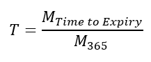
In the CBOE volatility index calculation methodology, time to expiration of a constituent option series, is calculated by dividing the number of minutes until expiration (MTime to Expiry) of the selected options (rounded down to the nearest minute) by the number of minutes in a year (M365).


VIX Time to Expiration Formula

Estimating the Forward Index Level

The next step is to estimate the forward index level of the S&P 500 using option markets prices. It represents the market’s expectation of the index value at expiration under the risk-neutral measure and serves as the reference point for selecting the relevant option contracts used in the calculation.

It is calculated using the principle of put-call parity, specifically by finding the unique strike price where the price difference between the call and the put option is at its absolute minimum.


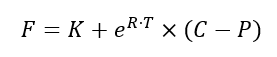
VIX Forward Price Formula

Where:

  • F: The forward index level
  • K: The smallest strike price at which the absolute difference between the call price and the put price is the smallest (|C – P| is minimized).
  • C: The market price (midpoint of the bid-ask spread) of the call option at the strike price Kmin.
  • P: The market price (midpoint of the bid-ask spread) of the put option at the strike price Kmin.
  • R: The risk-free interest rate (typically based on U.S. Treasury bills matching the option’s maturity).
  • T: The time to expiration (expressed as a fraction of a calendar year).

Determining K0

Once the forward index level has been estimated, we then identify K0, defined as the first strike price equal to or immediately below the forward index level (F). This strike acts as a reference point for the option selection process, separating the out-of-the-money put options from the out-of-the-money call options used in the calculation.

Selecting Out-of-the-Money Options

The VIX methodology uses a wide range of out-of-the-money (OTM) put and call options. OTM options are sensitive to changes in expected future volatility and provide information about the market’s expectations across a broad range of potential future outcomes. By incorporating both downside and upside option prices, the methodology captures the entire market-implied distribution of future index values rather than relying on a single option contract.

Variance Calculation

The Contribution of Individual Options Contracts

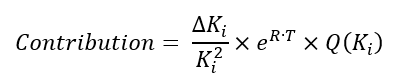
Each selected option contributes unique information about the market’s expectation of future variance. The weight of this contribution depends on three key factors: the option’s mid-price (Q(Ki)), the strike spacing (ΔKi) between neighbouring contracts, and the inverse square of its strike price (1/(Ki)2). This precise weighting scheme ensures that information from the entire out-of-the-money option chain is integrated into the final variance estimate.


VIX Option Contribution Formula

where for:


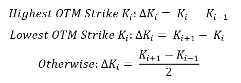
Strike Spacing Formula

The VIX Variance Formula

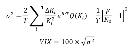
The option selection and weighting procedure described above is formally represented by the VIX variance formula. Rather than estimating volatility from a single option, the formula aggregates information from all selected option contracts to produce an estimate of expected future annualized variance.


VIX Variance Formula

Where:

  • σ2: Annualized variance
  • T: Time to expiration (in years)
  • F: Option-implied forward price
  • Ki: Strike price of the ith out-of-the-money option
  • K0: First strike equal to or otherwise immediately below the forward index level, F
  • ΔKi: Strike spacing for ith out-of-the-money option
  • Q(Ki): The mid-price of an option with strike Ki
  • R: Risk-free interest rate (with maturity equal to option expiration date)

Variance Estimates for Near-Term and Next-Term Options

Applying the variance formula to both the near-term and next-term options produces two separate estimates of expected future variance. The methodology calculates variance first because option portfolios can replicate future variance directly. As demonstrated by Demeterfi et al. (1999), a continuously weighted portfolio of out-of-the-money options across all strikes can replicate the payoff of a log contract, which is a theoretical derivative whose payout is tied to the logarithm of an asset’s price, making its returns purely dependent on variance rather than direction. Because a log contract captures total realized variance regardless of the asset’s price path, this foundational result allows expected future variance to be inferred directly and purely from observable option prices.

Constructing a Constant 30-Day Variance Measure

The variance estimates obtained from the near-term and next-term option maturities are linearly interpolated to obtain a constant 30-day estimate of annualized variance. Taking the square root converts variance into volatility, while multiplying by 100 expresses the result as a percentage. The resulting value is reported as the VIX index. The formula used in the interpolated CBOE volatility index calculation is as follows:


Interpolation Formula

Where:

  • MT1: The number of minutes until expiration of the near-term options
  • MT2: The number of minutes until expiration of the next-term options
  • MCM: The number of minutes in the given constant maturity term (30 days)
  • M365: The number of minutes in a 365-day year
  • Ti: MTi / M365
  • σi2: Variance of the i-th term

Interpretation of the VIX

For this section, we consider the S&P 500 index options data collected on June 18, 2026, with a spot price of $7,496.04 and a risk-free rate of 3.66%. Excel file with complete data and VIX calculations can be downloaded below.

Download the Excel file with complete dataset and VIX calculation

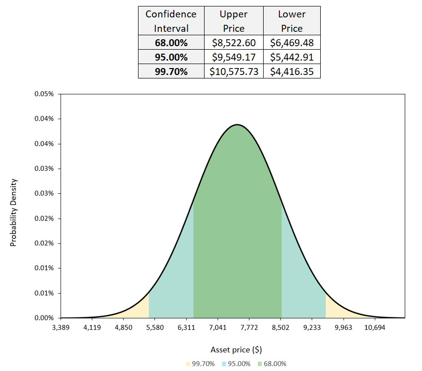
Our calculations yield a VIX value of 13.69, reflecting the market’s expectation of a ±13.69% movement over the next year. In Figure 1, we map this percentage onto a standard bell curve, where this expected movement in the S&P 500 index prices represent one standard deviation. This allows us to visualize the market’s expected range of price movements under the 68%, 95%, and 99.7% confidence intervals over the next one year.

Figure 1. Market Expected Price Over the Next 1 Year
Market Expected Price Over the Next 1 Year
Source: computation by the author.

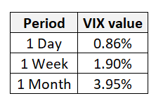
To calculate expected movements for shorter time frames, the VIX is scaled by dividing it by the square root of N, where N represents the number of periods in a year. For instance, N equals 12 to find a 1-month expected move, 52 for a 1-week move, and 252 trading days for a 1-day move.

Figure 2. Expected Movements for Shorter Time Frames
Expected Movements for Shorter Time Frames
Source: computation by the author.

You can download the Python code provided below, for VIX calculation using the modern CBOE methodology.

Download the Python code for VIX calculation.

Alternatively, you can download the R code below with the same functionality as in the Python file.

Download the R code for VIX calculation.

Why should I be interested in this post?

For anyone interested in finance or a career in trading, understanding how the VIX is constructed is crucial. As one of the most widely used measures of market uncertainty and expected volatility, it serves as an important tool for market analysis, risk assessment and numerous volatility-based trading strategies.

Related posts on the SimTrade blog

   ▶ Akshit GUPTA Options

   ▶ Jayati WALIA Black-Scholes-Merton Option Pricing Model

   ▶ Jayati WALIA Implied Volatility

   ▶ Saral BINDAL Implied Volatility and Option Prices

   ▶ Saral BINDAL Volatility curves: smiles and smirks

   ▶ Youssef LOURAOUI VIX index

Useful resources

Academic research

Black F. and M. Scholes (1973) The pricing of options and corporate liabilities. Journal of Political Economy, 81(3), 637–654.

Black, F. (1976), “Studies of Stock Price Volatility Changes”, Proceedings of the Business and Economics Section of the American Statistical Association, 177–181.

Britten-Jones, M. and A. Neuberger (2000) Option prices, implied price processes, and stochastic volatility. The Journal of Finance, 55(2), 839–866.

Demeterfi, K., Derman, E., Kamal, M., & Zou, J. (1999). A guide to volatility and variance swaps. The Journal of Derivatives, 6(4), 9-32.

Gârleanu, N., Pedersen, L. H., & Poteshman, A. M. (2009). Demand-based option pricing. The Review of Financial Studies, 22(11), 4259–4299.

Hull J.C. (2022) Options, Futures, and Other Derivatives, 11th Global Edition, Chapter 15 – The Black-Scholes-Merton model, 338–365.

Jiang, G. J. and Y. S. Tian (2005) The model-free implied volatility and its information content. The Review of Financial Studies, 18(4), 1305–1342.

Merton R.C. (1973) Theory of rational option pricing. The Bell Journal of Economics and Management Science, 4(1), 141–183.

Whaley, R. E. (1993). Derivatives on market volatility: Hedging tools long overdue. The Journal of Derivatives, 1(1), 71-84.

Business resources

Cboe Global Markets (February 26, 2026) Version 6.0 Cboe Volatility Index (VIX) Methodology.

Cboe Global Markets (February 26, 2026) Version 5.0 Cboe Volatility Index Mathematics Methodology.

About the author

The article was written in June 2026 by Saral BINDAL (Indian Institute of Technology Kharagpur, Metallurgical and Materials Engineering, 2024-2028 & Research assistant at ESSEC Business School). His interests include tracking geopolitical developments and analyzing their direct impact on macroeconomic factors such as inflation, trade balances, and currency volatility, with a focus on using data to quantify these global economic ripple effects.
Discover all posts written by Saral BINDAL.