

In this article, Saral BINDAL (Indian Institute of Technology Kharagpur, Metallurgical and Materials Engineering, 2024-2028 & Research assistant at ESSEC Business School) examines the statistical properties of historical VIX data and applies statistical methods to model its dynamics.
Introduction
The Chicago Board Options Exchange (CBOE) Volatility Index, or VIX, is a real-time market index designed to measure the market’s expectation of 30-day forward-looking annualized volatility in the US equity market. It is option-based, calculated using the market prices of S&P 500 index options to gauge expected volatility. The VIX construction methodology can be found in the article CBOE Volatility Index
In this article, we analyze the VIX index using historical market data to study its statistical properties, and discuss the methods used to model its dynamics in quantitative finance.
Historical Data
The VIX Index Historical data is publicly available from the Chicago Board Options Exchange (CBOE) and is updated on a daily basis. The analysis in this article is based on daily closing values of the VIX obtained from this data.
Figure 1 below illustrates the time series plot of VIX daily closing values from January 1990 to August 2026. From the figure, we can observe that during periods of high uncertainty, the VIX tends to rise significantly, as seen during the Global Financial Crisis (2007–2009) and the COVID-19 pandemic (2019–2020). We can also see the VIX rising as of now amid the ongoing Middle East crisis, although not to the same extent as observed during previous periods of heightened uncertainty.
Figure 1. VIX Index Historical Data (1990-2026)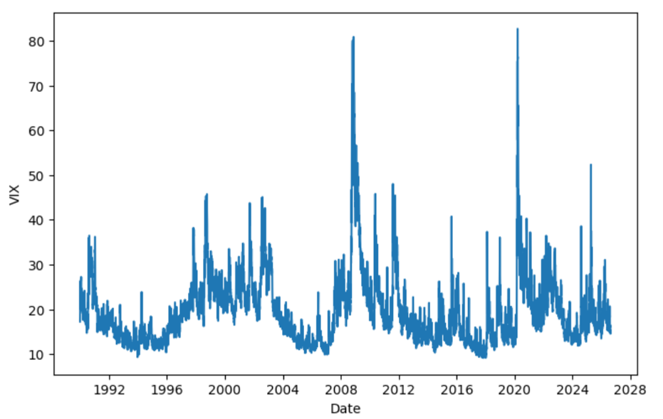
Source: computation by the author.
Distributional Characteristics
Using historical VIX data from 1990 to 2026, Figure 2 illustrates the empirical distribution of daily VIX closing values. The histogram, overlaid with a kernel density estimate (KDE), provides a visual representation of the distribution’s underlying probability density. The corresponding first four moments of the distribution are reported below:
Table 1. VIX Distribution Statistics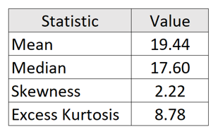
Source: computation by the author.
From the above table, we can observe that the data is right-skewed, which indicates that volatility tends to remain relatively low under normal market conditions but can rise sharply during periods of financial stress. The long right tail therefore reflects the occurrence of volatility shocks and tail-risk events, such as the Global Financial Crisis (2007–2009), the COVID-19 market shock (2020), and other episodes of significant financial or geopolitical uncertainty. Moreover, a high excess kurtosis indicates fatter tails compared to a normal distribution, implying a higher probability of observing extreme VIX levels. From the histogram, we observe that the VIX is concentrated around a level of 15 for a large proportion of the sample. This suggests that, under normal market conditions, the VIX tends to fluctuate around this level, which can be interpreted as its long-term level of the market uncertainty
Figure 2. Historical Distribution and Kernel Density Estimation of the Daily VIX levels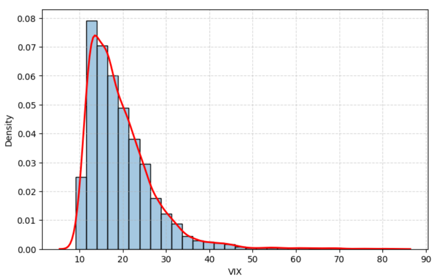
Source: computation by the author.
Time-Series Properties
The VIX exhibits several well-documented time-series properties that distinguish it from traditional financial asset prices. Unlike equity prices, whose levels are generally characterized by non-stationary dynamics, the VIX exhibits pronounced mean reversion and persistence, together with sharp spikes during episodes of market stress. The mean-reverting behaviour of the VIX is particularly noteworthy because it resembles a fundamental feature of interest-rate dynamics, which has long been incorporated into models such as the Vasicek (1977) and Cox, Ingersoll, and Ross (1985). The mean-reverting specifications have similarly been used to capture the tendency of volatility to return toward a long-run level.
However, the two processes differ substantially in their temporal dynamics. Interest-rate persistence typically reflects gradual adjustments in response to macroeconomic conditions and monetary policy, with mean reversion occurring over relatively longer horizons. In contrast, the VIX responds rapidly to changes in market expectations: episodes of financial stress can trigger abrupt upward spikes, followed by relatively rapid mean reversion toward lower levels. Thus, while both exhibit persistent and mean-reverting dynamics, the VIX is distinguished by its faster adjustment, pronounced asymmetry, and sharp responses to market stress.
Methods to Model VIX Dynamics
VIX dynamics exhibit several distinctive characteristics, particularly mean reversion and persistence, which require different modelling approaches. This section examines how various econometric models capture these features, ranging from mean-reverting and Log-VIX models to HAR, ARCH/GARCH, and stochastic volatility models.
Mean-Reverting Models
Early approaches to modelling volatility indices treated volatility as a mean-reverting stochastic process. A commonly used specification is the Cox-Ingersoll-Ross (CIR) process, originally developed for interest-rate modelling by Cox, Ingersoll and Ross (1985) and subsequently applied to volatility derivatives by Grünbichler and Longstaff (1996). Grünbichler and Longstaff modelled the volatility index using a mean-reverting square-root process and derived pricing formulas for volatility futures and options.
The dynamics are given by

- Vt represents the volatility index at time t
- κ is the speed of mean reversion
- θ is the long-run level towards which the process tends to revert
- σ is the diffusion parameter controlling the magnitude of random fluctuations
- Wt is a standard Brownian motion
The term κ(θ − Vt)dt represents the mean-reverting component, which pulls the process towards its long-run level θ, while σ√VtdWt represents the diffusion component, capturing random fluctuations in the volatility index.
The CIR framework was subsequently examined empirically in the context of VIX futures by Zhang and Zhu (2006). They estimated a stochastic variance model using historical VIX data and used it to derive and evaluate VIX futures prices.
An alternative mean-reverting modelling approach is the Ornstein-Uhlenbeck (OU) process (Uhlenbeck and Ornstein, 1930), which assumes a constant diffusion coefficient:

Unlike the CIR process, the OU process is Gaussian and can theoretically take negative values. This makes the OU process unsuitable for modelling the VIX level directly, since the VIX is strictly positive. A common way to retain the mean-reverting OU structure while ensuring a positive VIX is therefore to model log(VIX) rather than the VIX level itself.
Log-VIX Models
A natural way to address the possibility of negative values is to model the logarithm of the VIX. Let
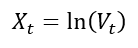
A mean-reverting logarithmic process can then be written as

or equivalently,

Since
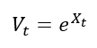
the resulting modelled VIX is strictly positive. The logarithmic transformation therefore preserves the mean-reverting structure while avoiding the negative-value problem associated with modelling the VIX level using a Gaussian process.
Mean-reverting in the log models were studied by Detemple and Osakwe (2000) in the context of volatility option valuation. Their model provides an early theoretical foundation for modelling volatility through a log-normal mean-reverting process. The approach was subsequently applied directly to the VIX by Bao (2013), who developed a mean-reverting logarithmic model for the spot VIX and extended it to incorporate jumps and stochastic volatility.
Heterogeneous Autoregressive Model
Although continuous-time mean-reverting models capture the tendency of volatility to move towards a long-run level, empirical evidence indicates that the VIX also exhibits substantial persistence across different time horizons. Fernandes, Medeiros and Scharth (2014) conducted a detailed analysis of the time-series properties of the VIX and found evidence of long-range dependence. They therefore employed Heterogeneous Autoregressive (HAR) models to model and forecast the VIX.
The HAR framework captures persistence by allowing past VIX observations over different horizons to affect the current value. A simplified HAR model can be expressed as

where
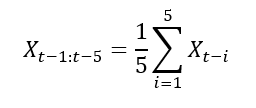
and
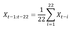
The three components represent information from daily, weekly, and monthly horizons, respectively. This allows the HAR-VIX model to capture the persistence of the VIX across different time horizons while remaining relatively simple and parsimonious. The HAR framework was originally introduced by Corsi (2009) to model the heterogeneous dynamics of realized volatility. Fernandes, Medeiros and Scharth (2014) adapted this framework to the VIX and showed that its multi-horizon structure provides a useful representation of the strong persistence and long-range dependence in the VIX.
Stochastic Variance of the VIX
The volatility of the VIX itself can vary over time. Rather than assuming that the diffusion coefficient is constant, stochastic-volatility models allow the volatility governing VIX fluctuations to evolve as a separate stochastic process.
Kaeck and Alexander (2013) investigate continuous-time models of VIX dynamics that explicitly incorporate stochastic volatility of volatility. Their analysis considers several one- and two-factor continuous-time models, including affine and non-affine specifications and models with jumps, using VIX data over an extended period.
Conceptually, the model can be represented as

where
- VIXt represents the VIX index
- Vt represents the instantaneous variance governing movements in log-VIX and is itself stochastic
- κ controls the mean-reversion speed of log-VIX
- θ represents the long-run level of log-VIX
- Wt is a Brownian motion driving log-VIX
- Zt represents the size of a jump in log-VIX
- Jt is a jump-counting process, with dJt representing the occurrence of jumps

- κv controls the mean-reversion speed of the variance process
- θv represents the long-run level of the variance process
- σv controls the volatility of the variance process, representing the volatility-of-volatility
- Wtv is a Brownian motion driving the variance process
The key distinction is therefore that the variance of VIX fluctuations is no longer constant. It becomes a state variable that evolves over time.
This additional source of randomness allows the model to capture changes in the intensity of VIX fluctuations and provides a more flexible representation of the sharp and persistent movements observed during periods of financial stress. Kaeck and Alexander’s analysis specifically examines whether stochastic volatility of volatility improves the ability of continuous-time models to describe VIX dynamics.
ARCH and GARCH Models
The VIX also exhibits volatility clustering, where periods of high volatility tend to be followed by high volatility, while periods of low volatility tend to be followed by low volatility. This suggests that the variance of log change in VIX is not constant over time. ARCH and GARCH models capture this feature by allowing the conditional variance of log change in VIX to evolve over time.
Let the log change in the VIX be defined as
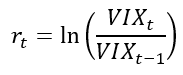
An ARCH or GARCH model can then be used to model the conditional variance of these changes. The standard GARCH(1,1) specification is

where
- rt represents the log change in the VIX at time t
- μ represents the conditional mean of the VIX log change
- εt represents the innovation or shock at time t
- σt2 represents the conditional variance of the VIX log change
- ω represents the long-run variance component
- α measures the immediate effect of new shocks on conditional variance
- β measures the persistence of conditional variance over time
The αεt−12 term captures the immediate impact of a new shock, while the βσt−12 term captures the persistence of previously elevated variance. A high value of β therefore indicates that periods of high variation in the VIX tend to persist.
The ARCH model was introduced by Engle (1982), while Bollerslev (1986) extended it to the more general GARCH framework. For the VIX, these models are useful for studying time-varying conditional variance and volatility clustering in VIX changes, rather than the mean-reverting behaviour of the VIX level itself.
Empirical Analysis of VIX
We use the complete historical daily VIX closing values (1990 – 2026) to estimate the parameters of the CIR model described above. Since the CIR model is specified in continuous time while the data are observed at daily intervals, the process is first discretized using the Euler-Maruyama approximation:

where Δt; = 1/252 for daily observations and εt+1 ∼ N(0,1). This discretization implies that, conditional on the previous day’s VIX value, the expected value and variance of the next observation are:
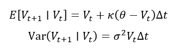
Assuming the discretized process is conditionally normally distributed, these expressions allow us to construct a likelihood for the observed VIX data. The log-likelihood is:

The CIR parameters are then estimated by choosing the values that maximize this log-likelihood:
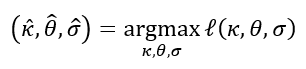
This gives an estimated mean-reversion speed of κ = 4.8618, a long-run VIX level of θ = 19.4237, and a diffusion parameter of σ = 5.1952.
These estimated parameters are then used to simulate a possible future path of the VIX. The simulation starts from the observed VIX value of 14.63 on 13th August 2026 and projects the VIX forward over 252 trading days using the CIR dynamics. The mean-reverting component pulls the process towards the estimated long-run level, while the diffusion component introduces random fluctuations around this tendency.
Figure 3 compares the historical VIX with one simulated path generated by the estimated CIR model. The historical series shows the large fluctuations and sharp spikes observed in the VIX over the sample period, while the simulated path represents one possible future realization starting from the current VIX level of 14.63. The dotted line at 19.42 represents the estimated long-run level of the VIX. The simulated path fluctuates around this level and exhibits a tendency to move towards it, illustrating the mean-reverting behavior implied by the CIR model.
You can download the Excel file with complete historical data used for the above calculations below.

Figure 3. Historical Path and Multiple CIR Simulated Paths for the VIX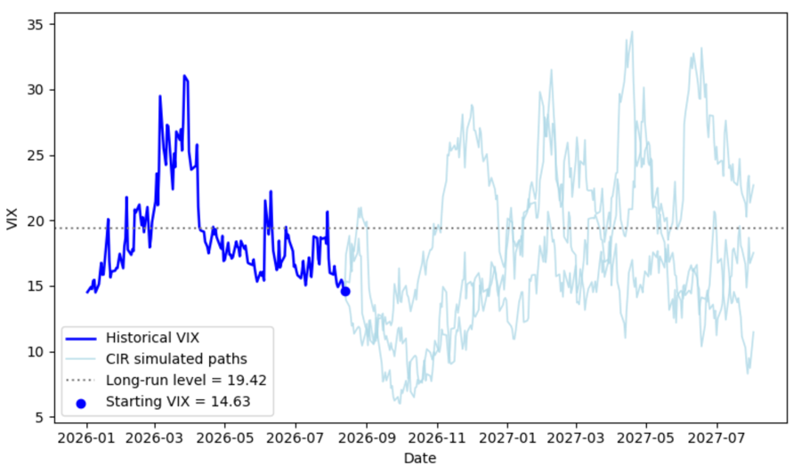
Source: computation by the author.
You can download the Python code below to reproduce the CIR parameter estimation and simulated VIX paths presented above.

Alternatively, you can download the R code below with the same functionality as in the Python file.

Why should I be interested in this post?
For anyone interested in finance or a career in trading, understanding the statistical properties of VIX and how it is modelled is very important. As one of the most widely used measures of market uncertainty and expected volatility, it serves as an important tool for market analysis, risk assessment and numerous volatility-based trading strategies.
Related posts on the SimTrade blog
▶ Akshit GUPTA Options
▶ Jayati WALIA Black-Scholes-Merton Option Pricing Model
▶ Jayati WALIA Implied Volatility
▶ Saral BINDAL Implied Volatility and Option Prices
▶ Saral BINDAL Volatility curves: smiles and smirks
▶ Youssef LOURAOUI VIX index
Useful resources
Academic research on option pricing
Black F. and M. Scholes (1973) The pricing of options and corporate liabilities. Journal of Political Economy, 81(3), 637-654.
Black, F. (1976), “Studies of Stock Price Volatility Changes”, Proceedings of the Business and Economics Section of the American Statistical Association, 177-181.
Cox J. C., J. E. Ingersoll and S. A. Ross (1985) A theory of the term structure of interest rates. Econometrica, 53(2), 385-407.
Hull J.C. (2022) Options, Futures, and Other Derivatives, 11th Global Edition, Chapter 15 – The Black-Scholes-Merton model, 338-365.
Merton R.C. (1973) Theory of rational option pricing. The Bell Journal of Economics and Management Science, 4(1), 141-183.
Uhlenbeck G. E. and L. S. Ornstein (1930) On the theory of the Brownian motion. Physical Review, 36(5), 823-841.
Academic research on VIX
Bao Q. (2013) Mean-Reverting Logarithmic Modelling of VIX. MPRA Paper, No. 46413.
Bollerslev T. (1986) Generalized autoregressive conditional heteroskedasticity. Journal of Econometrics, 31(3), 307-327.
Corsi F. (2009) A simple approximate long-memory model of realized volatility. Journal of Financial Econometrics, 7(2), 174-196.
Cox J. C., J. E. Ingersoll and S. A. Ross (1985) A theory of the term structure of interest rates. Econometrica, 53(2), 385-407.
Detemple J. and C. Osakwe (2000) The valuation of volatility options. European Finance Review, 4(1), 21-50.
Engle R. F. (1982) Autoregressive conditional heteroscedasticity with estimates of the variance of United Kingdom inflation. Econometrica, 50(4), 987-1007.
Fernandes M., M. C. Medeiros and M. Scharth (2014) Modelling and predicting the CBOE market volatility index. Journal of Banking & Finance, 40, 1-10.
Grünbichler A. and F. A. Longstaff (1996) Valuing futures and options on volatility. Journal of Banking & Finance, 20(6), 985-1001.
Jiang G. J. and Y. S. Tian (2005) The model-free implied volatility and its information content. The Review of Financial Studies, 18(4), 1305-1342.
Kaeck A. and C. Alexander (2013) Continuous-time VIX dynamics: On the role of stochastic volatility of volatility. International Review of Financial Analysis, 28, 46-56.
Uhlenbeck G. E. and L. S. Ornstein (1930) On the theory of the Brownian motion. Physical Review, 36(5), 823-841.
Whaley R. E. (2009) Understanding the VIX. Journal of Portfolio Management, 35(3), 98-105.
Zhang J. E. and Y. Zhu Y. (2006) VIX futures. Journal of Futures Markets, 26(6), 521-531.
VIX Data
CBOE Global Markets (2026) VIX Historical Data.
About the author
The article was written in September 2026 by Saral BINDAL (Indian Institute of Technology Kharagpur, Metallurgical and Materials Engineering, 2024-2028 & Research assistant at ESSEC Business School). His interests include tracking geopolitical developments and analyzing their direct impact on macroeconomic factors such as inflation, trade balances, and currency volatility, with a focus on using data to quantify these global economic ripple effects.
Discover all posts written by Saral BINDAL.