In this article, Youssef LOURAOUI (Bayes Business School, MSc. Energy, Trade & Finance, 2021-2022) presents the managed futures strategy (also called CTAs or Commodity Trading Advisors). The objective of the managed futures strategy is to look for market trends across different markets.
This article is structured as follow: we introduce the managed futures strategy principle. Then, we present the different types of managed futures strategies available. We also present a performance analysis of this strategy and compare it a benchmark representing all hedge fund strategies (Credit Suisse Hedge Fund index) and a benchmark for the global equity market (MSCI All World Index).
Introduction
According to Credit Suisse (a financial institution publishing hedge fund indexes), a managed futures strategy can be defined as follows: “Managed Futures funds (often referred to as CTAs or Commodity Trading Advisors) focus on investing in listed bond, equity, commodity futures and currency markets, globally. Managers tend to employ systematic trading programs that largely rely upon historical price data and market trends. A significant amount of leverage is employed since the strategy involves the use of futures contracts. CTAs do not have a particular biased towards being net long or net short any particular market.”
Managed futures funds make money based on the points below:
- Exploit market trends: trending markets tend to keep the same direction over time (either upwards or downwards)
- Combine short-term and long-term indicators: use of short-term and long-term moving averages
- Diversify across different markets: at least one market should move in trend
- Leverage: the majority of managed futures funds are leveraged in order to get increased exposures to a certain market
Types of managed futures strategies
Managed futures may contain varying percentages of equity and derivative investments. In general, a diversified managed futures account will have exposure to multiple markets, including commodities, energy, agriculture, and currencies. The majority of managed futures accounts will have a trading programme that explains their market strategy. The market-neutral and trend-following strategies are two main methods.
Market-neutral strategy
Market-neutral methods look to profit from mispricing-induced spreads and arbitrage opportunities. Investors that utilise this strategy usually attempt to limit market risk by taking long and short positions in the same industry to profit from both price increases (for long positons) and decreases (for short positions).
Trend-following strategy
Trend-following strategies seek to generate profits by trading long or short based on fundamental and/or technical market indicators. When the price of an asset is falling, trend traders may decide to enter a short position on that asset. On the opposite, when the price of an asset is rising, trend traders may decide to enter a long position. The objective is to collect gains by examining multiple indicators, deciding an asset’s direction, and then executing the appropriate trade.
Methodolgical isuses
The methodology to define a managed futures strategy is described below:
- Identify appropriate markets: concentrate on the markets that are of interest for this style of trading strategy
- Identify technical indicators: use key technical indicators to assess if the market is trading on a trend
- Backtesting: the hedge fund manager will test the indicators retained for the strategy on the market chosen using historical data and assess the profitability of the strategy across a sample data frame. The important point to mention is that the results can be prone to errors. The results obtained can be optimized to historical data, but don’t offer the returns computed historically.
- Execute the strategy out of sample: see if the in-sample backtesting result is similar out of sample.
This strategy makes money by investing in trending markets. The strategy can potentially generate returns in both rising and falling markets. However, understanding the market in which this strategy is employed, coupled with a deep understanding of the key drivers behind the trending patterns and the rigorous quantitative approach to trading is of key concern since this is what makes this strategy profitable (or not!).
Performance of the managed futures strategy
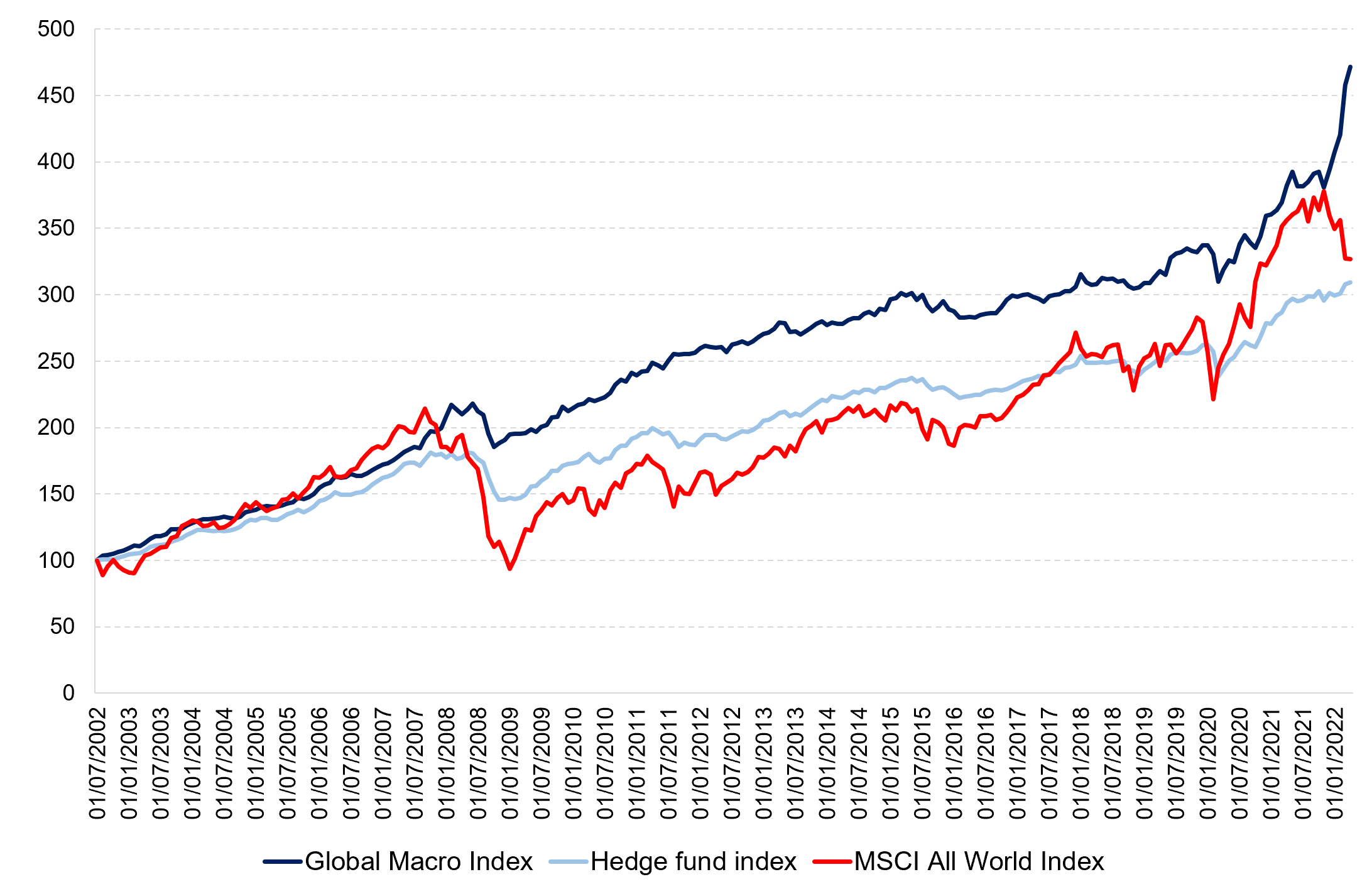
Overall, the performance of the managed futures strategy was overall not correlated from equity returns, but volatile (Credit Suisse, 2022). To capture the performance of the managed futures strategy, we use the Credit Suisse hedge fund strategy index. To establish a comparison between the performance of the global equity market and the managed futures strategy, we examine the rebased performance of the Credit Suisse managed futures index with respect to the MSCI All-World Index.
Over a period from 2002 to 2022, the managed futures strategy index managed to generate an annualized return of 3.98% with an annualized volatility of 10.40%, leading to a Sharpe ratio of 0.077. Over the same period, the Credit Suisse Hedge Fund Index managed to generate an annualized return of 5.18% with an annualized volatility of 5.53%, leading to a Sharpe ratio of 0.208. The managed futures strategy had a negative correlation with the global equity index, just about -0.02 overall across the data analyzed. The results are in line with the idea of global diversification and decorrelation of returns derived of the managed futures strategy from global equity returns.
Figure 1 gives the performance of the managed futures funds (Credit Suisse Managed Futures Index) compared to the hedge funds (Credit Suisse Hedge Fund index) and the world equity funds (MSCI All-World Index) for the period from July 2002 to April 2021.
Figure 1. Performance of the managed futures strategy.
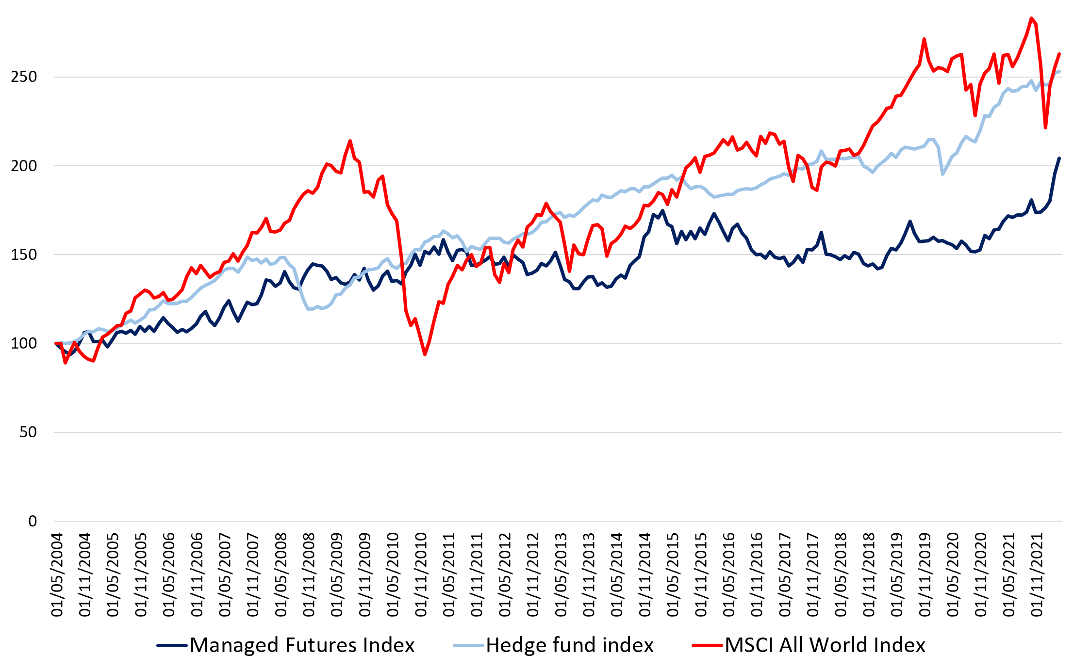
Source: computation by the author (Data: Bloomberg)
You can find below the Excel spreadsheet that complements the explanations about the Credit Suisse managed futures strategy.

Why should I be interested in this post?
Understanding the profits and risks of such a strategy might assist investors in incorporating this hedge fund strategy into their portfolio allocation.
Related posts on the SimTrade blog
▶ Youssef LOURAOUI Introduction to Hedge Funds
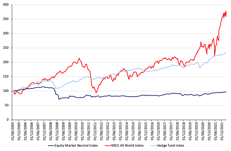
▶ Youssef LOURAOUI Equity market neutral strategy
▶ Youssef LOURAOUI Fixed income arbitrage strategy
▶ Youssef LOURAOUI Global macro strategy
▶ Youssef LOURAOUI Long/short equity strategy
▶ Youssef LOURAOUI Portfolio
Useful resources
Academic research
Pedersen, L. H., 2015. Efficiently Inefficient: How Smart Money Invests and Market Prices Are Determined. Princeton University Press.
Business Analysis
Credit Suisse Hedge fund strategy
Credit Suisse Hedge fund performance
Credit Suisse Managed futures strategy
Credit Suisse Managed futures performance benchmark
About the author
The article was written in January 2023 by Youssef LOURAOUI (Bayes Business School, MSc. Energy, Trade & Finance, 2021-2022).
 Source: computation by the author (Data: Bloomberg)
 Source: computation by the author. (Data: Reuters Eikon)