This article written by Akshit GUPTA (ESSEC Business School, Grande Ecole Program – Master in Management, 2019-2022) presents an introduction to Options.
Introduction
Options is a type of derivative which gives the buyer of the option contract the right, but not the obligation, to buy (for a call option) or sell (for a put option) an underlying asset at a price which is pre-determined, and a date set in the future.
Option contracts can be traded between two or more counterparties either over the counter or on an exchange, where the contracts are listed. Exchange based trading of option contracts was introduced to the larger public in April 1973, when Chicago Board Options Exchange (CBOE)) was introduced in the US. The options market has grown ever since with over 50 exchanges that trade option contracts worldwide.
Terminology used for an option contract
The different terms that are used in an option contract are:
Option Spot price
The option spot price is the price at which the option contract is trading at the time of entering the contract.
Underlying spot price
The underlying spot price is the price at which the underlying asset is trading at the time of entering the option contract.
Strike price
Strike price is essentially the price at which the option buyer can exercise his/her right to buy or sell the option contract at or before the expiration date. The strike price is pre-determined at the time of entering the contract.
Expiration date
The expiration date is the date at which the option contracts ends or after which it becomes void. The expiration date of an option contract can be set to be after weeks, months or year.
Lot size
A lot size is the quantity of the underlying asset contained in an option contract. The size is decided and amended by the exchanges from time to time. For example, an Option contract on an APPLE stock trading on an exchange in USA consists of 100 underlying APPLE stocks.
Option class
Option class is the type of option contracts that the trader is trading on. It can be a Call or a Put option.
Position
The position a trader can hold in an option contract can either be Long or Short depending on the strategy. A Long position essentially means Buying the option and a short position means Selling or writing the option contract.
Option Premium
Option premium is the price at which the option contracts trade in the market.
Benefits of using an option contract
Trading in option contracts gives the traders certain benefits which can be categorised as:
Hedging Benefits
Hedging is an essential benefit of the option contract. For an investor or a trader holding an underlying stock, an option contract provides them with the opportunity to offset their risk exposure by buying or selling an option contract as per their market outlook. If an trader holding stocks of APPLE is bearish about the market and expects the market to fall, he/she can buy a PUT option which essentially gives him/her the right to sell the security at a pre-determined price and date. Such a contract protects the trader from significant losses which he/she might incur if the stock price for APPLE goes down significantly.
Cost Benefits
While buying an option contract, the traders benefits from the leverage effect which exchanges across the world provides. Leverage helps the traders to multiply the size of their holdings with lesser capital investment. This also helps them to earn higher profits by taking limited risks.
Choice Benefits
In traditional trading, traders have a limited degree of flexibility as they can only buy or sell assets based on their outlook. Whereas, Option contracts provides a great choice to the traders as they can take different positions in call and put options (Long and short positions) and for different strikes and maturities.
They can also use different strategies and spreads to execute and manage their positions to earn profits.
Types of option contracts
The option contracts can be broadly classified into two categories: call options and put options.
Call options
A call option is a derivative contract which gives the holder of the option the right, but not an obligation, to buy an underlying asset at a pre-determined price on a certain date. An investor buys a call option when he believes that the price of the underlying asset will increase in value in the future. The price at which the options trade in an exchange is called an option premium and the date on which an option contract expires is called the expiration date or the maturity date.
For example, an investor buys a call option on Apple shares which expires in 1 month and the strike price is $90. The current apple share price is $100. If after 1 month,
The share price of Apple is $110, the investor exercises his rights and buys the Apple shares from the call option seller at $90.
But, if the share prices for Apple falls to $80, the investor doesn’t exercise his right and the option expires because the investor can buy the Apple shares from the open market at $80.
Put options
A put option is a derivative contract which gives the holder of the option the right, but not an obligation, to sell an underlying asset at a pre-determined price on a certain date. An investor buys a put option when he believes that the price of the underlying asset will decrease in value in the future.
For example, an investor buys a put option on Apple shares which expires in 1 month and the strike price is $110. The current apple share price is $100. If after 1 month,
The share price of Apple is $90, the investor exercises his rights and sell the Apple shares to the put option seller at $110.
But, if the share prices for Apple rises to $120, the investor doesn’t exercise his right and the option expires because the investor can sell the Apple shares in the open market at $120.
Different styles of option exercise
The option style doesn’t deal with the geographical location of where they are traded. However, the contracts differ in terms of their expiration time when they can be exercised. The option contracts can be categorized as per different styles they come in. Some of the most common styles of option contracts are:
American options
American style options give the option buyer the right to exercise his option any time prior or up to the expiration date of the contract. These options provide greater flexibility to the option buyer but also comes at a high price as compared to the European style options.
European options
European style options can only be exercised on the expiration or maturity date of the contract. Thus, they offer less flexibility to the option buyer in terms of his rights. However, the European options are cheaper as compared to the American options.
Bermuda options
Bermuda options are a mix of both American and European style options. These options can only be exercised on a specific pre-determined dates up to the expiration date. They are considered to be exotic option contracts and provide limited flexibility to the option buyer to exercise his claim.
Different underlying assets for an option contract
The different underlying assets for an option contract can be:
Individual assets: stocks, bonds
Option traders trading in individual assets can take positions in call or put options for equities and bonds based on the reports provided by the research teams. They can take long or short positions in the option contract. The positions depend on the market trends and individual asset analysis. The option contracts on individual assets are traded in different lot sizes.
Indexes: stock indexes, bond indexes
Options traders can also trade on contracts based on different indexes. These contracts can be traded over the counter or on an exchange. These traders generally follow the macroeconomic trends of different geographies and trade in the indices based on specific markets or sectors. For example, some of the most known exchange traded index options are options written on the CAC 40 index in France, the S&P 500 index and the Dow Jones Industrial Average Index in the US, etc.
Foreign currency options
Different banks and investment firms deal in currency hedges to mitigate the risk associated with cross border transactions. Options traders at these firms trade in foreign currency option contracts, which can be over the counter or exchange traded.
Option Positions
Option traders can take different positions depending on the type of option contract they trade. The positions can include:
Long Call
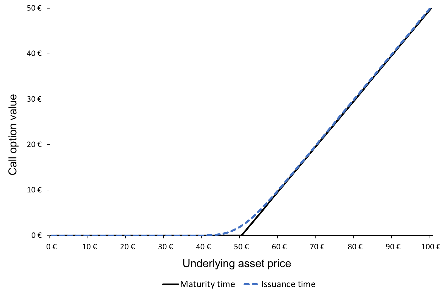
When a trader has a long position in a call option it essentially means that he has bought the call option which gives the trader the right to buy the underlying asset at a pre-determined price and date. The buyer of the call option pays a price to the option seller to buy the right and the price is called the Option Premium. The maximum loss to a call option buyer is restricted to the amount of the option premium he/she pays.
With the following notations:
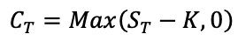
CT = Call option value at maturity T
ST = Price of the underlying at maturity T
K = Strike price of the call option
The graph of the payoff of a long call is depicted below. It gives the value of the long position in a call option at maturity T as a function of the price of the underlying asset at time T.
Payoff of a long position in a call option

Short Call
When a trader has a short position in a call option it essentially means that he has sold the call option which gives the buyer of the option the right to buy the underlying asset from the seller at a pre-determined price and date. The seller of the call option is also called the option writer and he/she receive a price from the option buyer called the Option Premium. The maximum gain to a call option seller is restricted to the amount of the option premium he/she receives.
With the following notations:
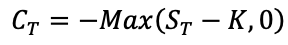
CT = Call option value at maturity T
ST = Price of the underlying at maturity T
K = Strike price of the call option
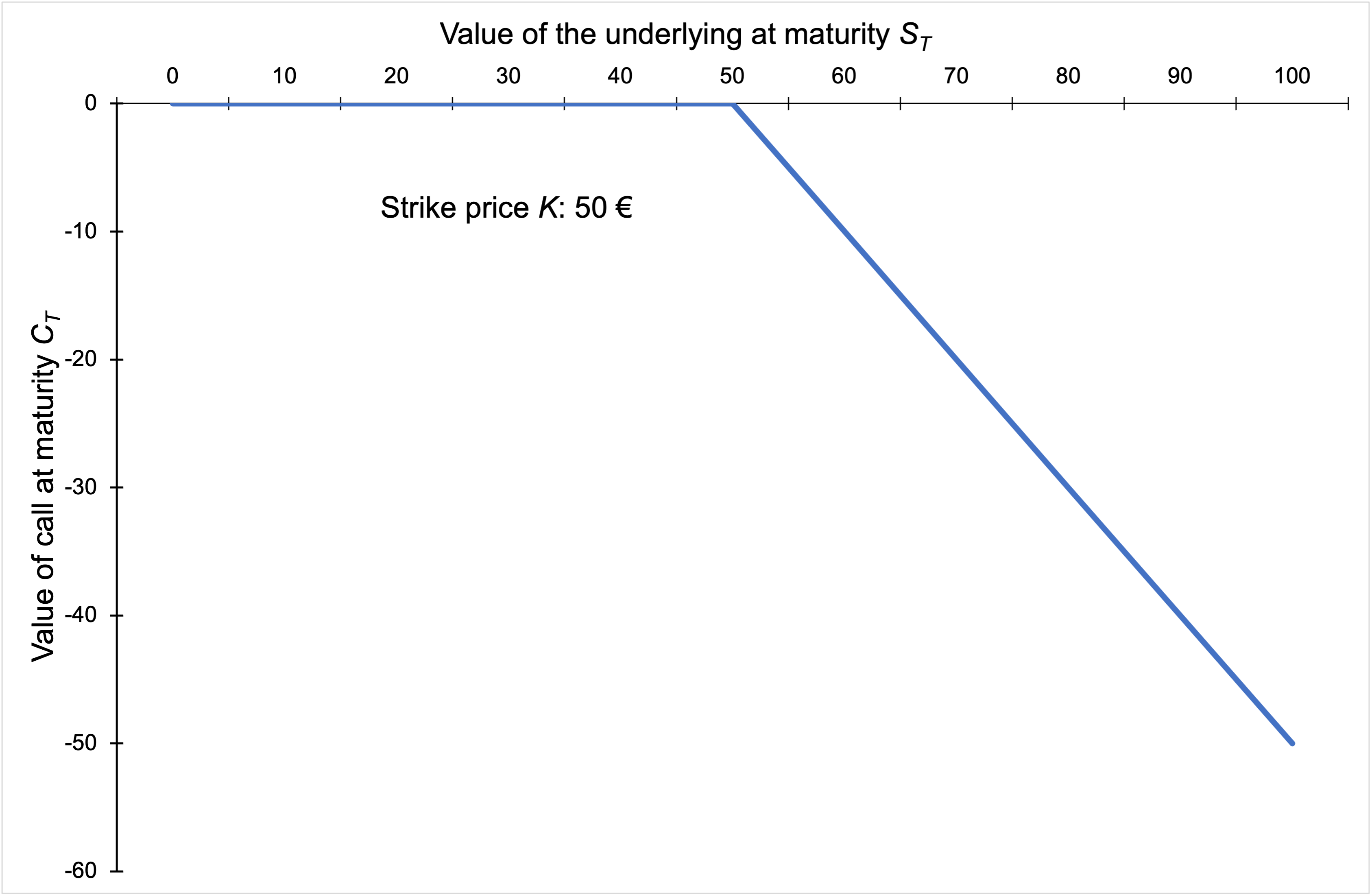
The graph of the payoff of a short call is depicted below. It gives the value of the short position in a call option at maturity T as a function of the price of the underlying asset at time T.
Payoff of a short position in a call option
Long Put
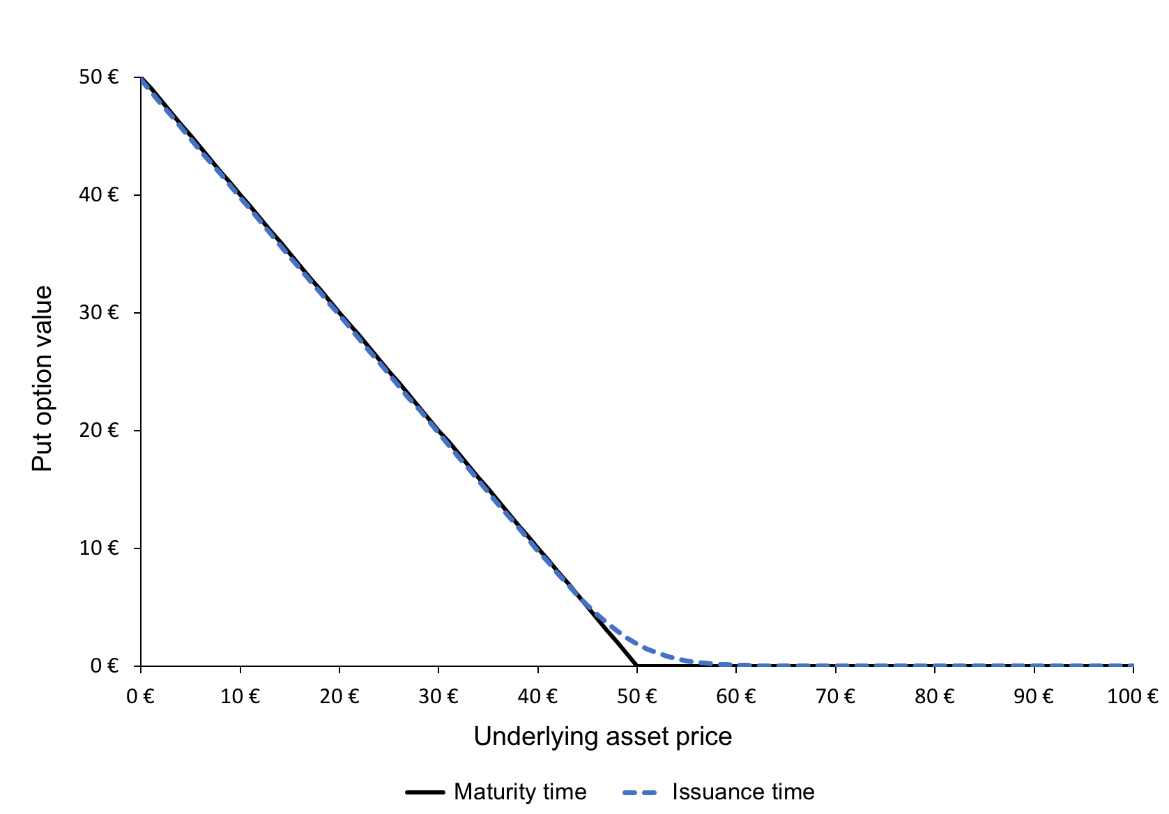
When a trader has a long position in a put option it essentially means that he/she has bought the put option which gives the trader the right to sell the underlying asset at a pre-determined price and date. The buyer of the put option pays a price to the option seller to buy the right and the price is called the Option Premium. The maximum loss to a put option buyer is restricted to the amount of the option premium he/she pays.
With the following notations:
PT = Put option value at maturity T
ST = Price of the underlying at maturity T
K = Strike price of the put option
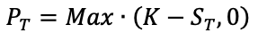
The graph of the payoff of a long put is depicted below. It gives the value of the long position in a put option at maturity T as a function of the price of the underlying asset at time T.
Payoff of a long position in a put option

Short Put
When a trader has a short position in a put option it essentially means that he has sold the call option which gives the buyer of the option the right to sell the underlying asset from the seller at a pre-determined price and date. The seller of the put option is also called the option writer and he/she receive a price from the option buyer called the Option Premium. The maximum gain to a put option seller is restricted to the amount of the option premium he/she receives.
With the following notations:
PT = Put option value at maturity T
ST = Price of the underlying at maturity T
K = Strike price of the put option
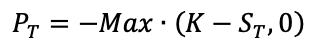
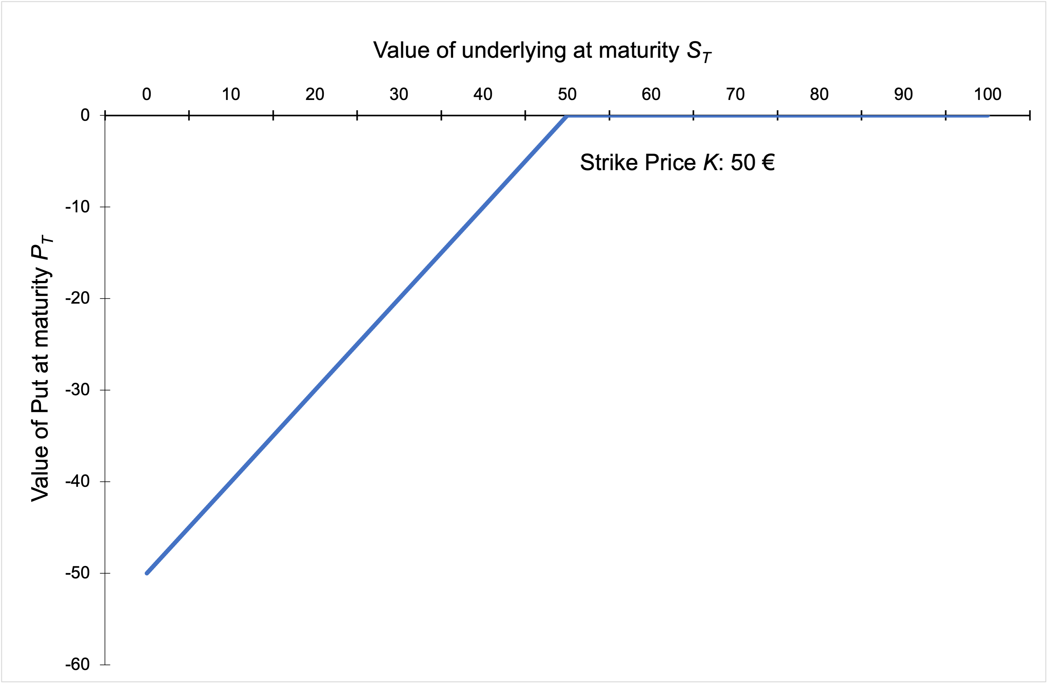
The graph of the payoff of a short put is depicted below. It gives the value of the short position in a put option at maturity T as a function of the price of the underlying asset at time T.
Payoff of a short position in a put option
Related posts on the SimTrade blog
▶ All posts about Options
▶ Jayati WALIA Black-Scholes-Merton option pricing model
▶ Akshit GUPTA Analysis of the Rogue Trader movie
▶ Akshit GUPTA History of Options markets
▶ Akshit GUPTA Option Trader – Job description
Useful Resources
Academic research
Hull J.C. (2015) Options, Futures, and Other Derivatives, Ninth Edition, Chapter 10 – Mechanics of options markets, 235-240.
Business analysis
CNBC Live option trading for APPLE stocks
About the author
Article written in June 2021 by Akshit GUPTA (ESSEC Business School, Grande Ecole Program – Master in Management, 2019-2022).