Value at Risk

Value at Risk

Jayati WALIA

In this article, Jayati WALIA (ESSEC Business School, Grande Ecole Program – Master in Management, 2019-2022) presents value at risk.

Introduction

Risk Management is a fundamental pillar of any financial institution to safeguard the investments and hedge against potential losses. The key factor that forms the backbone for any risk management strategy is the measure of those potential losses that an institution is exposed to for any investment. Various risk measures are used for this purpose and Value at Risk (VaR) is the most commonly used risk measure to quantify the level of risk and implement risk management.

VaR is typically defined as the maximum loss which should not be exceeded during a specific time period with a given probability level (or ‘confidence level’). Investments banks, commercial banks and other financial institutions extensively use VaR to determine the level of risk exposure of their investment and calculate the extent of potential losses. Thus, VaR attempts to measure the risk of unexpected changes in prices (or return rates) within a given period.

Mathematically, the VaR corresponds to the quantile of the distribution of returns on the investment.

VaR was not widely used prior to the mid 1990s, although its origin lies further back in time. In the aftermath of events involving the use of derivatives and leverage resulting in disastrous losses in the 1990s (like the failure of Barings bank), financial institutions looked for better comprehensive risk measures that could be implemented. In the last decade, VaR has become the standard measure of risk exposure in financial service firms and has even begun to find acceptance in non-financial service firms.

Computational methods

The three key elements of VaR are the specified level of loss, a fixed period of time over which risk is assessed, and a confidence interval which is essentially the probability of the occurrence of loss-causing event. The VaR can be computed for an individual asset, a portfolio of assets or for the entire financial institution. We detail below the methods used to compute the VaR.

Parametric methods

The most usual parametric method is the variance-covariance method based on the normal distribution.

In this method it is assumed that the price returns for any given asset in the position (and then the position itself) follow a normal distribution. Using the variance-covariance matrix of asset returns and the weights of the assets in the position, we can compute the standard deviation of the position returns denoted as σ. The VaR of the position can then simply computed as a function of the standard deviation and the desired probability level.

VaR Formula

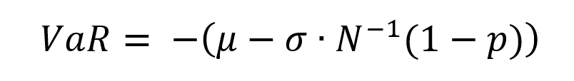
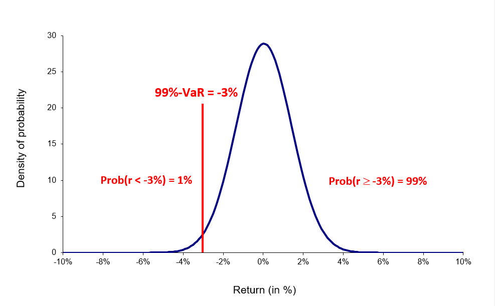
Wherein, p represents the probability used to compute the VaR. For instance, if p is equal to 95%, then the VaR corresponds to the 5% quantile of the distribution of returns. We interpret the VaR as a measure of the loss we observe in 5 out of every 100 trading periods. N-1(x) is the inverse of the cumulative normal distribution function of the confidence level x.

Figure 1. VaR computed with the normal distribution.

VaR computed with the normal distribution

For a portfolio with several assets, the standard deviation is computed using the variance-covariance matrix. The expected return on a portfolio of assets is the market-weighted average of the expected returns on the individual assets in the portfolio. For instance, if a portfolio P contains assets A and B with weights wA and wB respectively, the variance of portfolio P’s returns would be:

Variance of portfolio

In the variance-covariance method, the volatility can be computed as the unconditional standard deviation of returns or can be calculated using more sophisticated models to consider the time-varying properties of volatility (like a simple moving average (SMA) or an exponentially weighted moving average (EWMA)).

The historical distribution

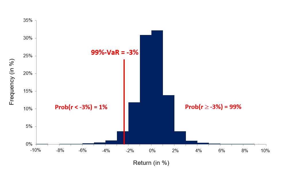
In this method, the historical data of past returns (for say 1,000 daily returns or 4 years of data) are used to build an historical distribution. VaR corresponds to the (1-p) quantile of the historical distribution of returns.
This methodology is based on the approach that the pattern of historical returns is indicative of future returns. VaR is estimated directly from data without estimating any other parameters hence, it is a non-parametric method.

Figure 2. VaR computed with the historical distribution.

VaR computed with the historical distribution

Monte Carlo Simulations

This method involves developing a model for generating future price returns and running multiple hypothetical trials through the model. The Monte Carlo simulation is the algorithm through which trials are generated randomly. The computation of VaR is similar to that in historical simulations. The difference only lies in the generation of future return which in case of the historical method is based on empirical data while it is based on simulated data in case of the Monte Carlo method.

The Monte Carlo simulation method is used for complex positions like derivatives where different risk factors (price, volatility, interest rate, dividends, etc.) must be considered.

Limitations of VaR

VaR doesn’t measure worst-case loss

VaR gives a percentage of loss that can be faced in a given confidence level, but it does not tell us about the amount of loss that can be incurred beyond the confidence level.

VaR is not additive

The combined VaR of two different portfolios may be higher than the sum of their individual VaRs.

VaR is only as good as its assumptions and input parameters

In VaR calculations especially parametric methods, unrealistic or inaccurate inputs can give misleading results for VaR. For instance, using the variance-covariance VaR method by assuming normal distribution of returns for assets and portfolios with non-normal skewness.

Different methods give different results

There are many approaches that have been defined over the years to estimate VaR. However, it essential to be careful in choosing the methodology keeping in mind the situation and characteristics of the portfolio or asset into consideration as different methods may be more accurate for specific scenarios.

Related posts on the SimTrade blog

   ▶ Jayati WALIA The variance-covariance method for VaR calculation

   ▶ Jayati WALIA The historical method for VaR calculation

   ▶ Jayati WALIA The Monte Carlo simulation method for VaR calculation

Useful Resources

Academic research articles

Artzner, P., F. Delbaen, J.-M. Eber, and D. Heath, (1999) Coherent Measures of Risk, Mathematical Finance, 9, 203-228.

Jorion P. (1997) “Value at Risk: The New Benchmark for Controlling Market Risk,” Chicago: The McGraw-Hill Company.

Longin F. (2000) From VaR to stress testing: the extreme value approach Journal of Banking and Finance, N°24, pp 1097-1130.

Longin F. (2016) Extreme events in finance: a handbook of extreme value theory and its applications Wiley Editions.

Longin F. (2001) Beyond the VaR Journal of Derivatives, 8, 36-48.

About the author

The article was written in September 2021 by Jayati WALIA (ESSEC Business School, Grande Ecole Program – Master in Management, 2019-2022).

Plain Vanilla Options

Plain Vanilla Options

Jayati WALIA

In this article, Jayati WALIA (ESSEC Business School, Grande Ecole Program – Master in Management, 2019-2022) presents plain vanilla options.

Introduction

An option contract is a financial derivative that gives its holder the right (but not the obligation) to trade an underlying asset at a price and a date set in advance.

In finance, plain vanilla refers to the most basic version of any financial instrument with standard features. Thus, a plain vanilla option simply refers to a contract that provides the option to buy or sell an underlying stock (or any financial asset) at a fixed price (known as the exercise/strike price) at an expiration date in the future. The expiration date (or maturity) of the option is the date when the holder can exercise her option if she wants.

In the US, options were first traded on an exchange on 26th April 1973. The Chicago Board Options Exchange (CBOE) was the first to create standardized, listed options. Today, there are over 50 exchanges worldwide that trade options.

When an option is bought, its holder pays a fixed amount to the option writer as the cost for the flexibility of trading that the option provides. This cost, which is essentially the value of an option (and the margin taken by the issuer), is known as the premium. The premium depends on the characteristics of the option like the strike price and the maturity, and on market data like the price of the underlying asset and especially its volatility. Many different underlying assets can be traded through options including stocks, bonds, commodities, foreign currencies.

Types of options

Vanilla options are of two types: call and put.

Call options

The holder of a call option has the right to buy a particular asset at a strike price K at maturity T. If the asset price at maturity denoted by ST is higher than K, then it is beneficial for the call option holder to exercise his option at time T as the price set in the call option contract K is lower than the market price ST. If the asset price at maturity ST is lower than K, then it is not beneficial for the call option holder to exercise his option at time T as the price set in the call option contract K is higher than the market price ST; he is then better off to buy the asset on the market at price ST than at price K.

For example, consider a call option on BNP Paribas stock with a strike price of €50 and a maturity date March 31st. The holder of this call option thus has the right but not the obligation to buy one BNP Paribas stock for €50 at maturity. He will exercise his option on March 31st if and only if the stock price is higher than €50.

The equation below gives the pay-off function of a call option that is the value of the call option at maturity T denoted by CT as a function of the price of the underlying asset ST.

Payoff formula for a call option

Figure 1 gives a graphical representation of the pay-off function of a call option that is the value of the call option at maturity T as a function of the price of the underlying asset at maturity T, ST, for a given strike price (equal to €50 in the figure).

Figure 1. Pay-off function of a call option

 Payoff for a call option

Put options

Similarly, the holder of a put option has the right to sell a particular asset at a strike price K at maturity T. If the asset price at maturity denoted by ST is higher than K, then it is beneficial for the put option holder not to exercise his option at time T as the price set in the put option contract K is lower than the market price ST; he is then better off to sell the asset on the market at price ST than at price K. If the asset price at maturity ST is lower than K, then it is beneficial for the put option holder to exercise his option at time T as the price set in the put option contract K is higher than the market price ST.

For example, consider a put option on BNP Paribas stock with a strike price of €50 and a maturity date March 31st. The holder of this put option thus has the right but not the obligation to sell one BNP Paribas stock for €50 at maturity. He will exercise his put option on March 31st if and only if the stock price is lower than €50.

The equation below gives the pay-off function of a put option that is the value of the put option at maturity T denoted by PT as a function of the price of the underlying asset ST.

Payoff formula for a put option

Figure 2 gives a graphical representation of the pay-off function of a put option that is the value of the put option at maturity T as a function of the price of the underlying asset ST for a given strike price (equal to €50 in the figure).

Figure 2. Pay-off function of a put option

 Payoff for a put option

Types of exercise

Options can be categorized based on their exercise restrictions.

American options

American options have the most flexible arrangement allowing holders to exercise their options at any time prior to the expiration date. They are widely traded over listed exchanges.

European options

European options provide less flexibility and allow holders to exercise options on only one specific date, which is the expiration date. They thus have a lower value compared to American options and are generally traded OTC.

Bermudan options

There are also Bermudan options that allow exercise of options on a set of specific dates before the expiration and thus provide holders a level of flexibility midway between American and European Options.

Moneyness

Options can also be characterized by their “moneyness” which compares the current price of the underlying asset to the option strike.

In-the-money options

An option with a positive intrinsic value is said to be ‘in the money’. This is the case for a call option if the current market price of the asset is higher than the strike price, and similarly for a put option if the current market price of the asset is lower than the strike price.

Out-of-the-money options

An option with a zero intrinsic value is said to be ‘out of the money’. This is the case for a call option if the current market price of the asset is lower than the strike price, and similarly for a put option if the current market price of the asset is higher than the strike price.

At-the-money options

An option with a strike price close or equal to the current market price is said to be ‘at the money’.

Option writers

The above discussion mainly revolves around option purchasers. However, there is also someone who is liable to sell (for a call) or buy (for a put) the underlying security whenever any holder exercises an option. The writer of an option is the person who is obligated to buy/sell the underlying in case of a call/put exercise. As a counterpart, the writer also receives the option premium from the holder.

The best-case scenario for a writer would be that the option is not exercised by its holder as the option remains out of the money (the writer earning the premium without being obliged to pay the cash flow at maturity). However, option writers are exposed to downside risks especially if the options they write are not covered i.e., holding a long or short position already in the underlying security depending on the option written.

Benefits

For traders with strong market views looking to leverage benefits from small to medium-term fluctuations in market price, buying options is an efficient means to offset their risk exposure. The buyer only risks a small amount of investment, and the downside is only limited to the initial premium whereas the upside is a high payoff if the speculation is in her/his favor. The traders can also take up multiple positions in different assets through options and leverage trade opportunities with profitable positions covering more than the hedging costs.

Option Trading

Most vanilla options are traded through exchanges that make it convenient to match buyers with sellers and vice versa. Trading of standardized contracts also promotes liquidity of the instruments in the market. Vanilla options generally come in series of standardized strike prices and expiration dates. For instance, for an option contract on an Apple Inc. stock (AAPL) expiring on 20th August 2021, the offered strike prices are $115, $120, $125, $130 and so on. Similarly, the expiration dates for listed stock options is generally the third Friday of the month in which the contract expires. If the Friday falls on a holiday, the expiration date becomes Thursday immediately before the third Friday.

Option pricing

The value an option is known at maturity as it is given by the contract. But what is the value of an option at the time of its issuance or at a time before maturity? Many mathematical models have been developed to answer this question. The most famous model is the Black-Scholes-Merton option pricing model. It uses a Brownian motion to model the behavior of stock market prices.

Use of options

Hedging

Options are commonly used in hedging. For instance, you can purchase an option on a stock to limit your losses to say 15% of your position, should the stock decline more than that during the option period.

Speculation

If one has a strong view about the potential market direction of an underlying security, one can make great returns on exploiting options, provided the view was right. This is essentially speculation in option trading. For instance, if you have a bullish opinion regarding a stock, you can purchase a call option on it that will allow you to purchase the stock at the strike price that will be lower than the future price (hopefully!). Thus, if you are right, you could exercise the option and your payoff would be the price difference between the stock price and the strike price. If you are wrong, you lose out on the premium you paid for the option.

Volatility

The volatility of the underlying asset affects positively option prices: stocks with higher volatility have more expensive option contracts that those with low volatility. In fact, the implied volatility (IV) of an option is that value of the volatility of the underlying instrument for which an option pricing model (such as the Black-Scholes-Merton model) will return a theoretical value equal to the current market price of that option. Hence, when the implied volatility increases, the price of options increases as well, assuming all other factors remain constant. When the implied volatility increases after a trade has been placed, it is good news for the option owner and, conversely bad news for the seller. Inversely, when the implied volatility decreases after a trade has been placed, it is bad news for the option owner and, conversely good news for the seller.

Note that the implied volatility tends to depend on the strike price and maturity date of the options for a given underlying asset. Once the implied volatility for the at-the-money contracts is determined in any given expiration month, market makers use pricing models and volatility skews to calculate implied volatility at other strike prices that are less heavily traded. So, every option has an associated volatility and risk profiles can vary drastically among options. Traders may at times balance out the risk of volatility by hedging one option with another.

Thus, it is essential to interpret and analyze risks before venturing into option trading. There are also many strategies that can be applied to vanilla options in order to benefit better and limit risk such as long and short calls/puts, bull and bear spreads, straddles and strangles, butterflies, condors among many.

Related posts on the SimTrade blog

All posts about Options

▶ Jayati WALIA Derivatives Market

▶ Jayati WALIA Black-Scholes-Merton option pricing model

▶ Jayati WALIA Brownian Motion in Finance

Useful Resources

Nasdaq Historical data for Apple stock

AVATRADE What are vanilla options

TheStreet Options Trading

About the author

The article was written in August 2021 by Jayati WALIA (ESSEC Business School, Grande Ecole Program – Master in Management, 2019-2022).

Derivatives Market

Derivatives Market

Jayati WALIA

In this article, Jayati WALIA (ESSEC Business School, Grande Ecole Program – Master in Management, 2019-2022) presents an overview of derivatives market.

Introduction

A financial market refers to a marketplace where various kinds of financial securities such as stocks, bonds, commodities, etc. are traded. The term ‘market’ can also refer to exchanges that are legal organizations that facilitate the trade of financial securities between buyers and sellers. In any case, these markets are categorized based of the type of financial securities that are traded through them. One such financial market is the Derivatives Market.

Derivatives market thus refers to the financial marketplace where derivative instruments such as futures, forwards and options contracts are traded between counterparties.

It was during the 1980s and 1990s that the financial markets saw a major growth in the trade of derivatives. A derivative is a financial instrument whose value is derived from the value of an underlying asset such as stocks, bonds, currencies, commodities, interest rates and/or different market indices. These underlying assets have fluctuating prices and returns, and derivatives provides a means to investors to reduce the risk exposure and leverage profits on these assets. Thus, derivatives are an essential class of financial instruments and central to the modern financial markets providing not just economic benefits but also resilience against risks. The most common derivatives include futures, forwards, options and swap contracts.

As per the European Securities and Markets Authority (ESMA), derivatives market has grown impressively (around 24 percent per year in the last decade) into a truly global market with over €680 trillion of notional amount outstanding. The interest rate derivatives (IRDs) accounted for 82% of the total notional amount outstanding followed by currency derivatives at 11%.

Main types of derivative contracts

Derivatives derive their value from an underlying asset, or simply an ‘underlying’. There is a wide range of financial instruments that can be an underlying for a derivative such as equities or equity index, fixed-income instruments, foreign currencies, commodities, and even other securities. And thus, depending on the underlying, derivative contracts can derive their values from corresponding equity prices, interest rates, foreign exchange rates, prices of commodities and probable credit events. The most common types of derivative contracts are elucidated below:

Forwards and Futures

Forward and futures contracts share a similar feature: they are an agreement between two parties to buy or sell a specified quantity of an underlying asset at a specified price (or ‘exercise price’) on a predetermined date in the future (or ‘expiration date’). While forwards are customized contracts i.e., they can be tailor-made according to the asset being traded, expiry date and price, and traded Over-the-Counter (OTC), futures are standardized contracts traded on centralized exchanges. The party that buys the underlying is said to be taking a long position while the party that sells the asset takes a short position and both parties are obligated to fulfil their part of the contract.

Options

An option contract is a financial derivative that gives its holder the right (but not the obligation) to trade an underlying asset at a price set in advance irrespective of the market price at maturity. When an option is bought, its holder pays a fixed amount to the option writer as cost for this flexibility of trading that the option provides, known as the premium. Options can be of the types: call (right to buy) or put (right to sell).

Swaps

Swaps are agreements between two counterparties to exchange a series of cash payments for a stated period of time. The periodic payments charged can be based on fixed or floating interest rates, depending on contract terms decided by the counterparties. The calculation of these payments is based on an agreed-upon amount, called the notional principal amount (or just notional).

Exchange-traded vs Over-the-counter Derivatives Market

Exchange-traded derivatives markets

Exchange-traded derivatives markets are standardized markets for derivatives trading and follows rules set by the exchange. For instance, the exchange sets the expiry date of the derivatives, the lot-size, underlying securities on which derivatives can be created, settlement process etc. The exchange also performs the clearing and settlement of trades and provide credit guarantee by acting as a counterparty for every trade of derivatives. Thus, exchanges provide a transparent and systematic course of action for any derivatives trade.

Over-the-counter markets

Over-the-counter (also known as “OTC”) derivatives markets on the other hand, provide a lesser degree of regulations. They were almost entirely unregulated before the financial crisis of 2007-2008 (also a time when derivatives markets were criticized, and the blame was placed on Credit Default Swaps). OTCs are customized markets and run by dealers who hedge risks by indulging in derivatives trading.

Types of market participants

The participants in the derivative markets can be categorized into different groups namely,

Hedgers

Hedging is a risk-neutralizing strategy when an investor seeks to protect a current or anticipated position in the market by limiting their risk exposure. They can do so by taking up an offset or counter position through derivative contracts. Parties such as individuals or companies who perform hedging are called Hedgers. The hedger thus aims to eliminate volatility against fluctuating prices of underlying securities and protect herself/himself from any downsides.

Speculators

Speculation is a very common technique used by traders and investors in the derivatives market. It is based on when traders have a strong viewpoint regarding the market behavior of any underlying security and though it is risky, if the viewpoint is correct, the speculation may reward with attractive payoffs. Thus, speculators use derivative contracts with a view to make profit from the subsequent price movements. They do not have any risk to hedge, in fact, they operate at a relatively high-risk level in anticipation of profits and provide liquidity in the market.

Arbitrageurs

Arbitrage is a strategy in which the participant (or arbitrageur) aims to make profits from the price differences which arise in the investments made in the financial markets as a result of mispricing. Arbitrageurs aim to earn low risk profits by taking two different positions in the same or different contracts (across different time periods) or on different exchanges to in-cash on price discrepancies or market inefficiencies.

Margin Traders

Margin is essentially the collateral amount deposited by an investor investing in a financial instrument to the counterparty in order to cover for the credit risk associated with the investment. In margin trading, the trader or investor is not required to pay the total value of your position upfront. Instead, they only need pay the margin amount which may vary and are usually fixed by the stock exchanges considering factors like volatility. Thus, margin traders buy and sell securities over a single session and square off their position on the same day, making a quick payoff if their speculations are right.

Criticism of derivatives

While derivatives provide numerous benefits and have significantly impacted modern finance and markets, they pose many risks too. In a 2002 letter to Berkshire Hathaway shareholders, Warren Buffet even described derivatives as “financial weapons of mass destruction”.

Derivatives are more highly leveraged due to relatively relaxed regulations surrounding them, and where one may need to put up half the money or more with buying other securities, derivatives traders can get by with just putting up a few percentage points of the total value of a derivatives contract as a margin. If the price of the underlying asset keeps falling, covering the margin account can lead to enormous losses. Derivatives are thus often criticized as they may allow investors to obtain unsustainable positions that elevates systematic risk so much that it can be equated to legalized gambling. Derivatives are also exposed to counterparty credit risk wherein there is scope of default on the contract by any of the parties involved in the contract. The risk becomes even greater while trading on OTC markets which are less regulated.

Derivatives have been associated with a number of high-profile credit events over the past two decades. For instance, in the early 1990s, Procter and Gamble Corporation lost more than $100 million in transactions in equity swaps. In 1995, Barings collapsed when one of its traders lost $1.4 billion (more than twice its then capital) in trading equity index derivatives.

The amounts involved with derivatives-related corporate financial distresses in the 2000s increased even more. Two such events were the bankruptcy of Enron Corporation in 2001 and the near collapse of AIG in 2008. The point of commonality among these events was the role of OTC derivative trades. Being an AAA-rated company, AIG was being exempted from posting collateral on most of its derivatives trading in 2008. In addition, AIG was unique among CDS market participants and acted almost exclusively as credit protection seller. When the global financial crisis reached its peak in late 2008, AIG’s CDS portfolios recorded substantial mark-to-market losses. Consequently, the company was asked to post $40 billion worth of collateral and the US government had to introduce a $150 billion financial package to prevent AIG, once the world’s largest insurer by market value, from filing for bankruptcy.

Conclusion

Derivatives were essentially created in response to some fundamental changes in the global financial system. If correctly handled, they help improve the resilience of the system, hedge market risks and bring economic benefits to the users. Thus, they are expected to grow further with financial globalization. However, past credit events have exposed many weaknesses in the organization of their trading. The aim is to minimize the risks associated with such trades while enjoying the benefits they bring to the financial system. An important challenge is to design new rules and regulations to mitigate the risks and to promote transparency by improving the quality and quantity of statistics on derivatives markets.

Related posts on the SimTrade blog

   ▶ All posts about Options

   ▶ Alexandre VERLET Understanding financial derivatives: options

   ▶ Jayati WALIA Plain Vanilla Options

   ▶ Alexandre VERLET Understanding financial derivatives: forwards

   ▶ Alexandre VERLET Understanding financial derivatives: futures

   ▶ Alexandre VERLET Understanding financial derivatives: swaps

Useful resources

Role of Derivatives in the 2008 Financial Crisis

ESMA Annual Statistical Report 2020

About the author

The article was written in August 2021 by Jayati WALIA (ESSEC Business School, Grande Ecole Program – Master in Management, 2019-2022).

Linear Regression

Linear Regression

Jayati WALIA

In this article, Jayati WALIA (ESSEC Business School, Grande Ecole – Master in Management, 2019-2022) presents linear regression.

Definition

Linear regression is a basic and one of the commonly used type of predictive analysis. It attempts to devise the relationship between two variables by fitting a linear function to observed data. A simple linear regression line has an equation of the form:


wherein Y is considered to be the dependent variable (i.e., variable we want to predict) and X is the explanatory variable (i.e., the variable we use to predict the dependent variable’s value). The slope of the line is β1, and β0 is the x-intercept. ε is the residual (or error) in prediction.

Application in finance

For instance, consider Apple stock (AAPL). We can estimate the beta of the stock by creating a linear regression model with the dependent variable being AAPL returns and explanatory variable being the returns of an index (say S&P 500) over the same time period. The slope of the linear regression function is our beta.

Figure 1 represents the return on the S&P 500 index (X axis) and the return on the Apple stock (Y axis), and the regression line given by the estimation of the linear regression above. The slope of the linear regression gives an estimate of the beta of the Apple stock.

Figure 1. Example of beta estimation for an Apple stock.

Beta_AAPL

Source: computation by the author (Data: Apple).

Before attempting to fit a linear model to observed data, it is essential to determine some correlation between the variables of interest. If there appears to be no relation between the proposed independent/explanatory and dependent, then the linear regression model will probably not be of much use in the situation. A numerical measure of this relationship between two variables is known as correlation coefficient, which lies between -1 and 1 (1 indicating positively correlated, -1 indicating negatively correlated, and 0 indicating no correlation). A popularly used method to evaluate correlation among the variables is a scatter plot.

The overall idea of regression is to examine the variables that are significant predictors of the outcome variable, the way they impact the outcome variable and the accuracy of the prediction. Regression estimates are used to explain the relationship between one dependent variable and one or more independent variables and are widely applied to domains in business, finance, strategic analysis and academic study.

Assumptions in the linear regression model

The first step in the process of establishing a linear regression model for a particular data set is to make sure that the in consideration can actually be analyzed using linear regression. To do so, our data set must satisfy some assumptions that are essential for linear regression to give a valid and accurate result. These assumptions are explained below:

Continuity

The variables should be measured at a continuous level. For example, time, scores, prices, sales, etc.

Linearity

The variables in consideration must share a linear relationship. This can be observed using a scatterplot that can help identify a trend in the relationship of variables and evaluate whether it is linear or not.

No outliers in data set

An outlier is a data point whose outcome (or dependent) value is significantly different from the one observed from regression. It can be identified from the scatterplot of the date, wherein it lies far away from the regression line. Presence of outliers is not a good sign for a linear regression model.

Homoscedasticity

The data should satisfy the statistical concept of homoscedasticity according to which, the variances along the best-fit linear-regression line remain equal (or similar) for any value of explanatory variables. Scatterplots can help illustrate and verify this assumption

Normally-distributed residuals

The residuals (or errors) of the regression line are normally distributed with a mean of 0 and variance σ. This assumption can be illustrated through a histogram with a superimposed normal curve.

Ordinary Least Squares (OLS)

Once we have verified the assumptions for the data set and established the relevant variables, the next step is to estimate β0 and β1 which is done using the ordinary least squares method. Using OLS, we seek to minimize the sum of the squared residuals. That is, from the given data we calculate the distance from each data point to the regression line, square it, and calculate sum of all of the squared residuals(errors) together.

Thus, the optimization problem for finding β0 and β1 is given by:

After computation, the optimal values for β0 and β1 are given by:

Using the OLS strategy, we can obtain the regression line from our model which is closest to the data points with minimum residuals. The Gauss-Markov theorem states that, in the class of conditionally unbiased linear estimators, the OLS estimators are considered as the Best Linear Unbiased Estimators (BLUE) of the real values of β0 and β1.

R-squared values

R-squared value of a simple linear regression model is the rate of the response variable variation. It is a statistical measure of how well the data set is fitted in the model and is also known as coefficient of determination. R-squared value lies between 0 and 100% and is evaluated as:

The greater is the value for R-squared, the better the model fits the data set and the more accurate is the predicted outcome.

Useful Resources

Linear regression Analysis

Simple Linear Regression

Related Posts

   ▶ Louraoui Y. Beta

About the author

The article was written in August 2021 by Jayati WALIA (ESSEC Business School, Grande Ecole – Master in Management, 2019-2022).

Quantitative Finance: Introduction and Scope

Quantitative Finance: Introduction and Scope

Jayati WALIA

In this article, Jayati WALIA (ESSEC Business School, Grande Ecole – Master in Management, 2019-2022) presents an overview of Quantitative Finance.

Quantitative Finance: Introduction and Scope

Quantitative finance has become an integral part of modern finance with the advent of innovative technologies, trading platforms, mathematical models, and sophisticated algorithms. In lay man terms, it is essentially the application of high-level mathematics and statistics to finance problems. Quantitative finance majorly focuses on most frequently traded securities. The very basis of it involves observation and quantitative analysis of market prices (stock prices, exchange rates, interest rates, etc.) over time, along with applying them to stochastic models and deducing results to make security pricing, trading, risk assessment, hedging and many other investment decisions. Hence, the heavy involvement of mathematics and especially stochastic calculus. However, it is not limited to that. In fact, theories and concepts from many other disciplines including physics, computer science, etc. have contributed to put together what we know as quantitative finance today.

Brief History

It was in the 20th century that the foundations of Quantitative Finance were laid starting off with the ‘Theory of Speculation’ PhD thesis by the French mathematician Louis de Bachelier. Bachelier applied the concept of Brownian motion to asset price behavior for the first time. Later the Japanese mathematician Kiyoshi Îto wrote a paper on stochastic differential equations and founded the stochastic calculus theory that is also named after him (Îto calculus) and is widely used in option pricing. The major breakthrough however, came in the 1970s when Robert Merton’s ‘On the pricing of corporate debt: the risk structure of interest rates’ and Fischer Black and Myron Scholes’ ‘The pricing of options and corporate liabilities’ research papers were published which inherently presented a call and put option pricing model and after that there was no looking back. The Black-Sholes-Merton model known as “BSM” model is widely used and is creditable for the boom of the options market. Today many more stochastic models have been devised to extend the BSM model, setting the benchmarks of quantitative analysis higher and benefitting the global economy.

Market participants

Quantitative Finance is used by many market participants: banks, financial institutions, investors and businesses who want better and automated control over their finances given the fluctuating behavior of the assets they trade. Initially, quantitative finance was majorly used in modelling market finance problems like pricing and managing derivative products for trading, managing risk of the investments in contracts, etc. basically in the sell-side of the firms such as Investment Banking. However, with continuous advancements, we see increased usage in buy-side as well among areas like Hedge Funds and Asset Management through development of quantitative models to analyze asset behavior and predict market movements in order to leverage potential trading opportunities.

Thus, any firm or investor that deals in financial derivatives (futures and options), portfolios of stocks and/or bonds, etc. need to use Quantitative Finance. These participants have specialized analysts to work on the quantitative finance and they are generally known as Quantitative Analysts or ‘quants’. Once referred to as ‘the rocket scientists of Wall Street’, quants have sound understanding of finance, mathematics and statistics combined with the acumen of programming/coding. With the dramatic changes in industry witnessed over the past years, quants with a stellar combination of the mentioned disciplines are greatly in demand.

Types of Quants

Quants create and apply financial models for derivative pricing, market prediction and risk mitigation. There are however many variations in quant roles, some of which are explained below:

  • Front Office Quant: Work in proximity with traders and salespersons on the trade floor. Implement pricing models used by traders to spot out new opportunities and provide guidance on risk strategies.
  • Quant Researcher: Essentially the Back Office quants, they research and design high frequency algorithms, pricing models and strategies for traders and brokerage firms.
  • Quant Developer: They are essentially software developers in a financial firm. They translate business requirements provided by researchers into code applications.
  • Risk Management Quant: They build models for keeping in check credit and regulatory operations and assessing credit risk, market risk, ALM (Asset and Liability Management) risk etc. They are the Middle Office quants and perform risk analysis of markets and assets and stress testing of the models too.

The Future of Quantitative Finance

Quants and Quantitative finance are here to stay! With firms becoming larger than life and the tremendous data and money involved, the scope and demand for quantitative finance is escalating like never before. Quantitative Finance is no more just about complex mathematics and stochastic models. With finance becoming more technical, data science, machine and deep learning and artificial intelligence are taking over the domain’s informative decision-making strategies. Thus, quantitative finance is being driven to new heights by the power of high processing computer algorithms that enable us to analyze enormous data and run model simulations within nanoseconds. To quote Rob Arnott, American entrepreneur and founder of Research Affiliates: “To a man with a hammer, everything looks like a nail. To a quant, anything that can’t be quantified is ignored. And historical data is our compass, even though we know that past performance is no guarantee of future results.”

Useful resources

Quantitative Finance
What is Quantitative Finance?
2020 Quants predict next decade in global finance

Related Posts

About the author

The article was written in July 2021 by Jayati WALIA (ESSEC Business School, Grande Ecole – Master in Management, 2019-2022).

Fixed-income products

Fixed-income products

Jayati WALIA

In this article, Jayati WALIA (ESSEC Business School, Grande Ecole – Master in Management, 2019-2022) presents fixed-income products.

Introduction

Fixed-income products are a type of debt securities that provides predetermined returns to investors in terms of a principle amount at maturity and/or interest payments paid periodically up to and including the maturity date (also known as coupon payments). For investors, fixed-income securities pay out a fixed set of cashflows that are known in advance and are hence preferred by conservative investors with low-risk appetite or those looking to diversify their portfolio and limit risk exposure. For companies and governments issuing these securities, it is a mechanism to raise capital to fund operations and projects.

The most elementary type of fixed-income instrument is the coupon-bearing bond. The values of different bonds depend on the coupon size, maturity date and market view of future interest rate behaviours (or essentially bond market yields). For eg., prices of bonds with longer maturity fluctuate more by interest rate changes. Bonds are generally traded OTC unlike equity stocks that are traded via exchanges. The risk exposure of a bond can be gauged by their Credit Rating issued by rating agencies (S&P, Moody’s, Fitch). The least risky bonds have a rating of AAA which indicates a high measure of credit worthiness and minimum degree of default.

Fixed-income products can come in many forms as well which include single securities like treasury bills, government bonds, certificate of deposits, commercial papers and corporate bonds, and also mutual funds and structured products such as asset back securities.

Types of fixed-income products

Fixed-income products come in several structures catering to the needs of investors and issuers. The most common types are explored below in detail:

Treasury bills

Treasury bills (also called “T-bills”) are money market instruments that are issued by governments with a short maturity ranging from one month to one year. These bills are used to fund short-term financing needs of governments and are backed by the Treasury Department. They are issued at discounted value and redeemed at par value. The difference between the issuance and redemption price is the net gain or income for the investor. The T-Bills are generally issued in denomination of $1,000 per bill. For example, if you buy a T-bill issued by the US Department of Treasury with a maturity of 52 weeks at $990, you will redeem your T-bill at a price of $1,000 upon maturity.

Treasury notes and bonds

Treasury notes and bonds are a type of fixed-income security issued by governments with a medium or long maturity beyond one year. These bonds are used to fund permanent financial needs of governments and are backed by the Treasury Department. They come with predetermined interest payments. They are considered to be the safest investment since they are backed by the government. As a consequence, government bonds come with low returns. Government bonds are usually traded over the counter (OTC) markets. Technically, government bonds come in various forms: zero-coupon bonds, fixed payment and inflation protected securities.

Corporate bonds

Corporate bonds, as the name suggests, are issued by corporations to finance their investments. They generally come with higher yields as compared to the government bonds as they are perceived as more risky investments. The expected return for such bonds generally depends on the company’s financial situation reflected in its credit rating. Corporations can issue different types of bonds which includes zero-coupon bonds, floating-rate bonds, convertible bonds, perpetual bonds, and subordinated bonds.

Asset-backed securities

Asset-backed securities (ABS) is a kind of fixed-income product that comprises of multiple debt pools packaged together as a single security (also known as ‘securitization’) and sold to investors. The assets that can be securitized include home loans (mortgages), auto loans, student loans, credit card receivables among others. Thus the interest and principal payments made by consumers of the individual debts are passed on to the investors as the yield earned on the ABS.

Benefits of fixed-income products

For issuers

Generally, fixed-income products are issued by governments and corporations to raise capital for their operation.

For firms, the issuance of bonds in financial markets along with bank credit (two types of debt) allows firms to use leverage. Interests can also be deduced from income such that the firm will pay less taxes.

For investors

The investment in fixed-income products is considered to be a conservative strategy as it presents low returns (compared to stocks) but also provides a relatively low-risk exposure. Other benefits include:

  • Capital protection: Fixed income products carry less risk as compared to other asset classes such as stocks. These investments ensure capital preservation till the maturity of the investment and are preferred by investors who are risk averse and look for stable returns.
  • Generation of predetermined income: The income from fixed-income products is generated by means of interest or coupon payments. The income level for such products is predetermined at the time of investment and is paid on a regular basis (usually semi-annually or annually). Also, investors benefit from income tax exemption on investment in many fixed-income products.
  • Seniority rights: The holders of corporate bonds get seniority rights in terms of repayment of their capital if the company goes into bankruptcy.
  • Diversification: The fixed-income markets are less sensitive to market risk compared to the equity markets. So, the fixed-income products are considered to be less risky than the equity market investments and generally provides a fixed or stable stream of income. To manage the risk exposure for any portfolio, investors prefer investing in fixed income products to diversify their investments and offset any losses which may result from the equity markets.

Risks associated with fixed-income products

While fixed-income securities are considered to provide relatively low risk exposure, volatility in the bond market may still prove tricky. Bond value and interest rates have an inverse relationship and increase in interest rates thus affects the bond value negatively. Due to the fixed coupon rate and interest payments, fixed-income securities are highly sensitive to inflation rates as cashflows may lose value. There is also credit risk including potential default by the issuer. If an investor buys international bonds, she/he is always exposed to exchange risk due to the ever-fluctuating FX rates.

Thus it is essential for investors to take into account these factors and purchase fixed-income securities according to their individual requirements and risk appetite.

Useful resources

Amodeo K. (10/05/20201) Fixed Income Explanation, Types, and Impact on Economy The Balance.

Blackrock Education: What is fixed income investing?

Corporate Fiannce Institute: Fixed-income securities

Related posts

About the author

The article was written by Jayati WALIA (ESSEC Business School, Grande Ecole – Master in Management, 2019-2022).