In this article, Alexandre LANGEVIN (ESSEC Business School, Global Bachelor in Business Administration (BBA), 2022-2026) examines why retail option strategies frequently underperform — that is, generate returns below a passive buy-and-hold benchmark or lose money outright — despite offering payoff profiles that appear attractive on paper. The article explains the structural mechanics behind four common strategies, identifies the sources of systematic drag, and illustrates how the gap between theoretical upside and realized performance emerges even before behavioral factors are considered.
Introduction
Options are among the most versatile yet complex instruments in financial markets. They can hedge risk, generate income, or express a directional view with defined downside (Hull, 2012). Yet a growing body of evidence suggests that retail investors who trade options systematically underperform both the market and their own expectations (Barber and Odean, 2000; de Silva, So and Smith, 2024). The question is not whether options are useful tools; they plainly are. The question is whether the specific strategies retail investors tend to favor are structurally suited to delivering the outcomes they expect.
The answer, in most cases, is that they are not. The gap between the payoff diagram and realized performance is not primarily attributable to adverse price realizations. It is embedded in the mechanics of how options are priced, how time erodes their value, and how the probability of profit is systematically lower than the shape of the payoff curve implies. Understanding these mechanics is the first step toward using options more deliberately.
How an Option Payoff Works
An option gives its buyer the right, but not the obligation, to buy (call) or sell (put) an underlying asset at a fixed price — the strike — on or before expiry. The buyer pays a premium for this right. At expiry, the profit or loss is determined entirely by the final price of the underlying relative to the strike.
For a long call: the option expires worthless if the underlying finishes below the strike. Above the strike, the buyer receives the difference between the final price and the strike. The buyer pays the premium upfront when entering the position; profit or loss at expiry therefore equals the intrinsic value minus this initial cost. The breakeven is therefore the strike plus the premium. For a long put, the logic is symmetric: the option has value if the underlying falls below the strike, and the breakeven is the strike minus the premium. Throughout this article, net profit or loss refers to the outcome at expiry after accounting for the premium paid upfront. The net profit or loss formula for a long call is:

These payoff diagrams look appealing. The downside is capped at the premium paid; the upside is theoretically unlimited for calls and capped at the strike price minus the premium paid for puts (since the underlying cannot fall below zero) for puts. What the diagram does not show is the probability attached to each outcome.
The Four Strategies: Structure and Mechanics
The Excel model accompanying this article covers four strategies commonly used by retail investors. Each illustrates a distinct structural trade-off.
The following four strategies represent the most common approaches used by retail option traders, ranging from directional speculation to income generation.
Long Out-of-the-Money (OTM) Call. An option is out-of-the-money when exercising it immediately would produce no value — the strike is above the current price for a call, or below it for a put. In the illustrative example, SPY trades at $540. A call with a $560 strike costs $5.20. Breakeven is $565.20, requiring a 4.7% move in the underlying just to recover the premium. Below $560 at expiry, the entire $5.20 is lost. Above $565.20, the trade turns profitable. The net profit or loss is positively skewed and theoretically unlimited, which explains its appeal. The structural problem is that an OTM call requires the underlying to move by more than the market already expects, because the premium reflects that expected move.
A worked example illustrates the arithmetic. Suppose SPY closes at $575 at expiry. The intrinsic value of the $560 call is $575 − $560 = $15. Net profit per share = $15 − $5.20 = $9.80, or $980 per contract (one contract = 100 shares) — a return of 188% on the premium paid. Now suppose SPY closes at $550 instead. The call expires worthless; the loss is the full premium of $5.20 per share, or −$520 per contract. These two outcomes — $980 profit vs. −$520 loss — illustrate the asymmetry. The upside is real, but the full loss scenario is far more probable: SPY must rise more than 4.7% simply to break even, and more than that to generate meaningful profit.
Long OTM Put. A $520 put on SPY trading at $540 costs $4.80. Breakeven is $515.20, requiring a 4.6% decline. Like the OTM call, the put must overcome both the out-of-the-money gap and the premium cost before generating any return. In calm markets, the probability of hitting breakeven by expiry is well below what the payoff diagram implies.
Bull Call Spread. Buying the $550 call and selling the $570 call reduces the net cost to $5.30 (long premium $8.50 minus short premium $3.20). Breakeven falls to $555.30, and maximum profit is capped at $14.70 per share if SPY finishes above $570. The spread trades unlimited upside for a lower entry cost and a higher probability of profit compared to the naked call. The payoff formula is:

It is a more disciplined structure, but it still requires a meaningful directional move, and the profit ceiling is fixed regardless of how far the underlying moves above the upper strike.
Covered Call. An investor who holds 100 shares purchased at $540 sells a $560 call for $5.20. Breakeven falls from $540 to $534.80. If SPY finishes below $560, the investor keeps the premium and the position. If SPY finishes above $560, the shares are called away and the investor captures only $25.20 per share in total profit, regardless of how far the stock has risen. The strategy generates income but structurally caps the upside.
Figure 1. Payoff diagrams at expiry for the four strategies (illustrative inputs).
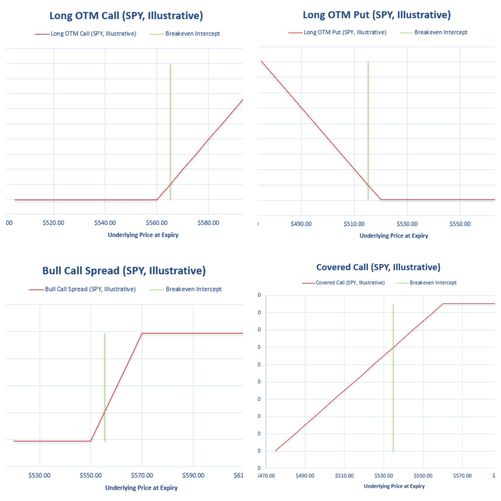
Source: computation by the author.
The Structural Sources of Underperformance
Three structural factors — theta decay, the volatility risk premium, and breakeven mechanics — explain why retail option strategies systematically underperform, independently of any behavioral bias.
Theta decay. Options lose value over time as expiry approaches. This decay is not linear; it accelerates sharply in the final weeks before expiry. A 30-day option that has lost 30% of its value in the first two weeks may lose the remaining 70% in the last two. Retail investors who buy short-dated options and hold them without a clear exit plan are running against the clock. The underlying must move quickly and decisively; a slow drift in the right direction is often not enough to overcome the daily erosion in time value. De Silva, So and Smith (2024) document that retail investors systematically purchase options ahead of anticipated volatility spikes, only to suffer double-digit percentage losses as volatility collapses and time value erodes post-announcement.
The volatility risk premium. Implied volatility — the level of volatility priced into an option’s premium — is persistently higher than realized volatility on average. This gap is the volatility risk premium, and it represents a systematic transfer of wealth from option buyers to option sellers. When you buy an option, you are paying for a level of volatility that, on average, does not materialize. Market makers and institutional sellers collect this premium consistently over time; retail buyers pay it. Broadie, Chernov and Johannes (2009) show that the apparently large returns to put-selling strategies are fully explained by compensation for bearing this volatility risk — what looks like alpha is largely a risk premium that option buyers are systematically on the wrong side of.
Breakeven mechanics. The breakeven calculation makes the structural difficulty explicit. For a long OTM call with a 4.7% breakeven requirement, the underlying must rise by 4.7% before expiry simply to recover costs. Historically, the probability of a large-cap equity index moving 5% or more in a given month is well below 50%. The payoff diagram shows what happens if the move occurs; it does not show how often it does. Most retail option buyers look at the profit region of the diagram without adequately pricing in the probability of reaching it. Barber and Odean (2000) document a closely related pattern in equity trading: retail investors systematically overestimate their ability to generate above-market returns, a bias that is amplified in options markets by the apparent leverage and lottery-like payoffs.
Transaction costs and taxes. A fourth source of drag, often overlooked, is the cost of trading itself. Retail investors typically pay per-contract commissions, and bid-ask spreads on options are wide relative to the premium — particularly for short-dated or illiquid contracts. On a $5.20 premium, a $0.10 spread represents nearly 2% of the position cost before any price move occurs. Capital gains taxes on short-term option profits further reduce net returns. These costs do not appear on payoff diagrams but compound the structural disadvantages described above.
Excel Model
The Excel model below contains four sheets — Long OTM Call, Long OTM Put, Bull Call Spread, and Covered Call — each following the same structure: an input table with yellow input cells, a payoff table across a range of expiry prices, and a payoff diagram with a breakeven marker. All inputs are illustrative and can be modified freely. The payoff columns and chart update automatically when inputs change.
Figure 2. Bull Call Spread sheet: inputs table and payoff formula.
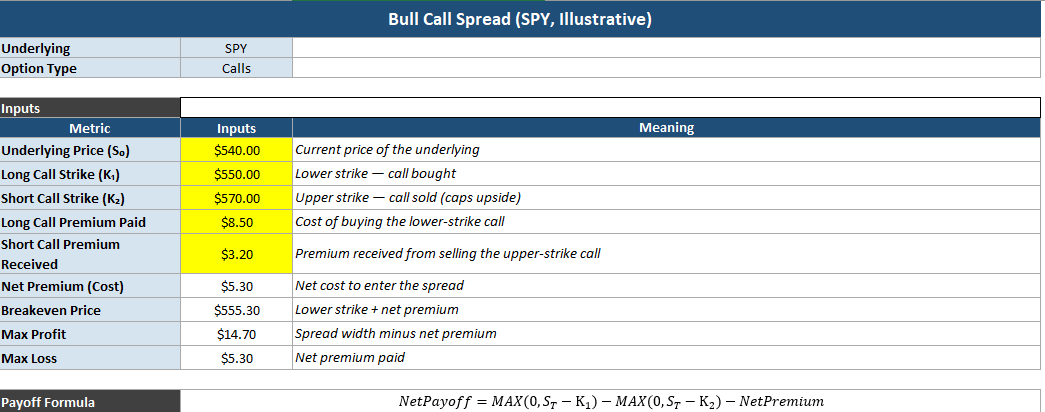
Source: computation by the author.

Why should I be interested in this post?
Options appear in equity research, derivatives desk interviews, and structured product discussions at banks and asset managers. Beyond the professional context, understanding why certain strategies structurally underperform is relevant for anyone who trades independently or advises clients on portfolio construction. The payoff diagram is the beginning of the analysis, not the end. Knowing how to read the probability distribution behind it is what separates informed use from speculation.
Related posts on the SimTrade blog
▶ Shengyu ZHENG Pricing barrier options with simulations and sensitivity analysis with Greeks
▶ Luis RAMIREZ Understanding Options and Options Trading Strategies
▶ Alexandre VERLET Understanding financial derivatives: options
▶ Saral BINDAL Implied Volatility and Option Prices
▶ All posts about Financial techniques
Useful resources
Academic research
Barber, B.M. and Odean, T. (2000) Trading Is Hazardous to Your Wealth: The Common Stock Investment Performance of Individual Investors, Journal of Finance, 55(2), 773-806. Available at https://faculty.haas.berkeley.edu/odean/papers%20current%20versions/individual_investor_performance_final.pdf
de Silva, T., So, E.C. and Smith, K. (2024) Losing is Optional: Retail Option Trading and Expected Announcement Volatility, Review of Finance, 30(2), 489-535. Available at https://www.timdesilva.me/files/papers/losing_optional.pdf
Broadie, M., Chernov, M. and Johannes, M. (2009) Understanding Index Option Returns, Review of Financial Studies, 22(11), 4493-4529. Available at https://business.columbia.edu/sites/default/files-efs/pubfiles/3964/broadie_chernov_johannes.pdf
Hull, J.C. (2012) Options, Futures, and Other Derivatives, 8th edition, Pearson.
About the author
This post was written in April 2026 by Alexandre LANGEVIN (ESSEC Business School, Global Bachelor in Business Administration (BBA), 2022-2026). Alexandre is interested in derivatives markets, options trading, and quantitative approaches to portfolio analysis.
▶ Discover all articles by Alexandre LANGEVIN.