Leverage in LBOs: How Debt Creates and Destroys Value in Private Equity Transactions

Ian DI MUZIO

In this article, Ian DI MUZIO (ESSEC Business School, Master in Finance (MiF), 2025–2027) explores the economics of leverage in leveraged buyouts (LBOs) from an investment banking perspective.

Rather than treating debt as a purely mechanical input in an Excel model, the article explains—both conceptually and technically—how leverage amplifies equity returns, reshapes risk, affects pricing, and constrains deal execution.

The ambition is to provide junior analysts with a realistic framework they can use when building or reviewing LBO models during internships, assessment centres, or live mandates.

Context and objective

Most students encounter leverage for the first time through a simplified capital structure slide: a bar divided into senior debt, subordinated debt, and equity, followed by a formula showing that higher debt and lower equity mechanically increase the internal rate of return (IRR, the discount rate that sets net present value to zero).

In the abstract, the story appears straightforward. If a company generates stable cash flows, a sponsor can finance a large share of the acquisition with relatively cheap debt, repay that debt over time, and magnify capital gains on a smaller equity cheque.

In reality, this mechanism operates only within a narrow corridor. Too little leverage and the financial sponsor struggles to compete with strategic buyers. Too much leverage and the business becomes fragile: covenants tighten, financial flexibility disappears, and relatively small shocks in performance can wipe out the equity.

The objective of this article is therefore not to restate textbook identities, but to describe how investment bankers think about leverage when advising financial sponsors and corporate sellers, drawing on market practice and transaction experience (see, for example, Kaplan & Strömberg).

The focus is on the interaction between free cash flow generation, debt capacity, pricing, and exit scenarios, and on how analysts should interpret LBO outputs rather than merely producing them.

What an LBO really is

At its core, a leveraged buyout is a change of control transaction in which a financial sponsor acquires a company using a combination of equity and a significant amount of borrowed capital, secured primarily on the target’s own assets and cash flows.

The sponsor is rarely a long-term owner. Instead, it underwrites a finite investment horizon—typically four to seven years—during which value is created through a combination of operational improvement, deleveraging, multiple expansion, and sometimes add-on acquisitions, before exiting via a sale or initial public offering emphasises.

From a financial perspective, an LBO is effectively a structured bet on the spread between the company’s return on invested capital and the cost of debt, adjusted for the speed at which that debt can be repaid using free cash flow.

In other words, leverage only creates value if operating performance is sufficiently strong and stable to service and amortise debt. When performance falls short, the rigidity of the capital structure becomes a source of value destruction rather than enhancement.

How leverage amplifies equity returns

The starting point for understanding leverage is the identity that equity value equals enterprise value minus net debt. If enterprise value remains constant while net debt declines over time, equity value must mechanically increase.

This is the familiar deleveraging effect: as free cash flow is used to repay borrowings, the equity slice of the capital structure expands even if EBITDA growth is modest and exit multiples remain unchanged.

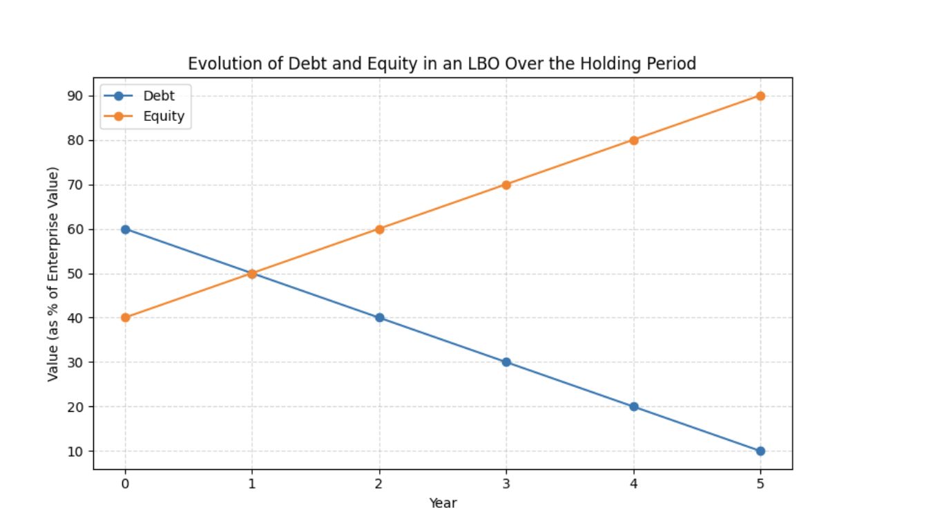
Figure 1 illustrates this mechanism in a stylised LBO. The company is acquired with high initial leverage. Over the holding period, EBITDA grows moderately, but the primary driver of equity value creation is the progressive reduction of net debt.

Figure 1. Evolution of capital structure in a simple LBO.
 Evolution of capital structure in a simple LBO
Source: the author.

Figure 1 illustrates the evolution of capital structure in a simple LBO. Debt is repaid using free cash flow, causing the equity portion of enterprise value to increase even if valuation multiples remain unchanged.

To enhance transparency and pedagogical value, the Excel model used to generate Figure 1—allowing readers to adjust leverage, cash flow, and amortisation assumptions—can be made available alongside this article.

This dynamic explains why LBO IRRs can appear attractive even with limited operational growth. It also highlights the fragility of highly levered structures: when EBITDA underperforms or exit multiples contract, equity value erodes rapidly because the initial leverage leaves little margin for error.

Debt capacity and the role of free cash flow

For investment bankers, the key practical question is not “how much leverage maximises IRR in Excel?” but “how much leverage can the business sustainably support without breaching covenants or undermining strategic flexibility?”.

This shifts the focus from headline EBITDA to the quality, predictability, and cyclicality of free cash flow. In an LBO context, free cash flow is typically defined as EBITDA minus cash taxes, capital expenditure, and changes in working capital, adjusted for recurring non-operating items.

A business with recurring revenues, limited capex requirements, and stable working capital can support materially higher leverage than a cyclical, capital-intensive company, even if both report similar EBITDA today.

Debt capacity is assessed using leverage and coverage metrics such as net debt to EBITDA, interest coverage, and fixed-charge coverage, tested under downside scenarios rather than a single base case. Lenders focus not only on entry ratios, but on how those ratios behave when EBITDA compresses or capital needs spike.

Pricing, entry multiples, and the leverage trade-off

Leverage interacts with pricing in a non-linear way. At a given entry multiple, higher leverage reduces the equity cheque and tends to increase IRR, provided exit conditions are favourable.

However, aggressive leverage also constrains bidding capacity. Lenders rarely support structures far outside market norms, which means sponsors cannot indefinitely substitute leverage for price. In competitive auctions, sponsors must choose whether to compete through valuation or capital structure, knowing that both dimensions feed directly into risk.

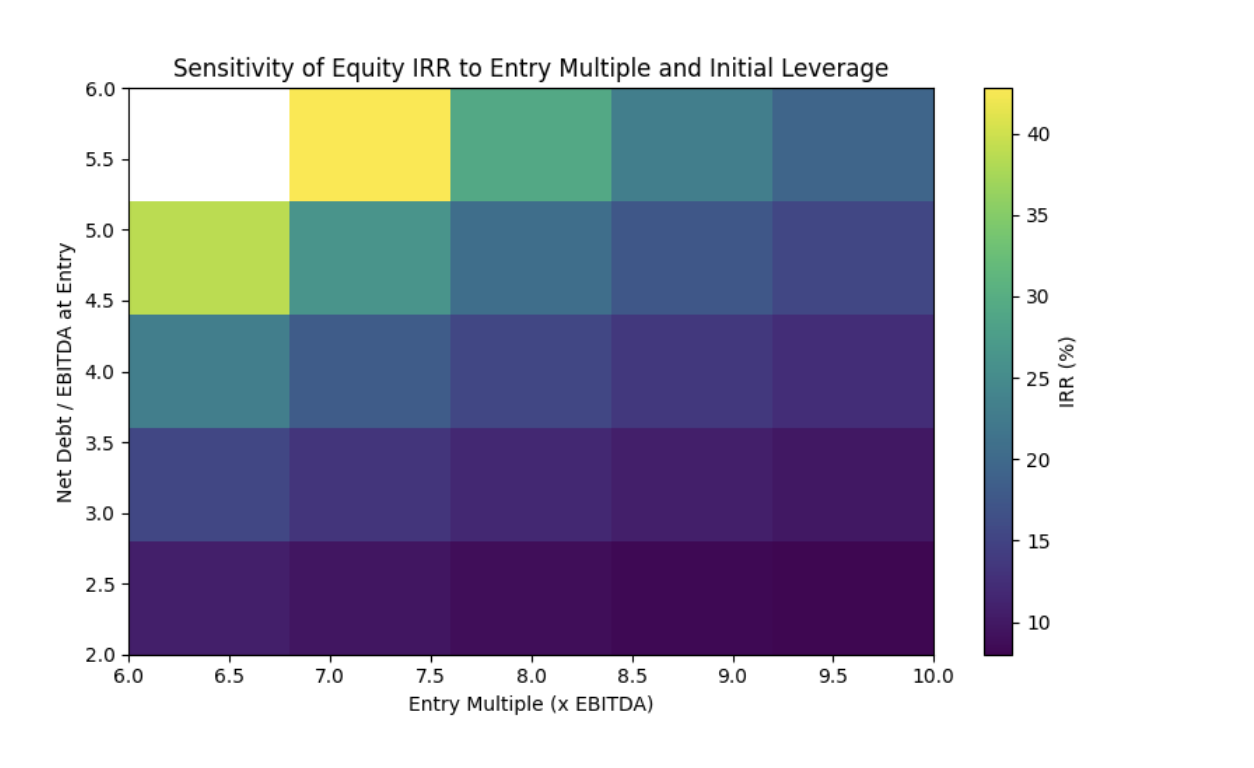
Figure 2 presents a stylised sensitivity of equity IRR to entry multiple and starting leverage, holding exit assumptions constant.

Figure 2. Sensitivity of equity IRR to entry valuation and starting leverage.
 Sensitivity of equity IRR to entry valuation and starting leverage
Source: the author.

Figure 2 illustrates the sensitivity of equity IRR to entry valuation and starting leverage. Outside a moderate corridor, IRR becomes highly sensitive to small changes in operating or exit assumptions.

Providing the Excel file behind Figure 2 would allow readers to stress-test entry pricing and leverage assumptions interactively.

Risk, scenarios, and the distribution of outcomes

A mature view of leverage focuses on the full distribution of outcomes rather than a single base case. Downside scenarios quickly reveal how leverage concentrates risk: when performance weakens, equity absorbs losses first.

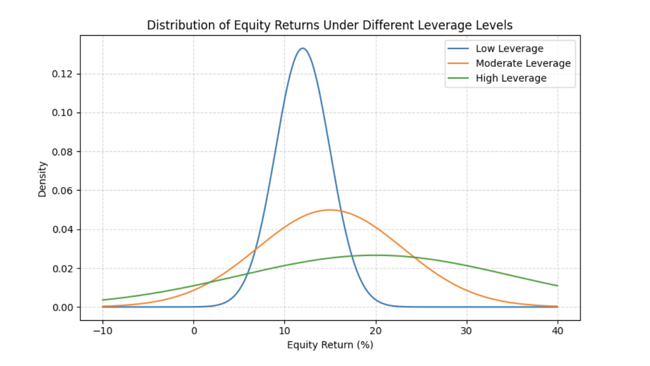
Figure 3 illustrates how higher leverage increases expected IRR but also widens dispersion, creating both a fatter upside tail and a higher probability of capital loss.

Figure 3. Distribution of equity returns under low, moderate, and high leverage.
Distribution of equity returns under low, moderate, and high leverage
Source: the author.

Higher leverage raises expected returns but materially increases downside risk.

For junior bankers, the key lesson is that leverage is a design choice with consequences. A robust analysis interrogates downside resilience, covenant headroom, and the coherence between capital structure and strategy.

The role of investment banks

Investment banks play a central role in structuring and advising on leverage. On buy-side mandates, they assist sponsors in negotiating financing packages and ensuring proposed leverage aligns with market appetite. On sell-side mandates, they help sellers compare bids not only on price, but on financing certainty and execution risk.

Conclusion

Leverage sits at the heart of LBO economics, but its effects are often oversimplified. For analysts, the real skill lies in linking model outputs to a coherent economic narrative about cash flows, debt service, and downside resilience.

Related posts on the SimTrade blog

   ▶ Alexandre VERLET Classic brain teasers from real-life interviews

   ▶ Emanuele BAROLI Interest Rates and M&A: How Market Dynamics Shift When Rates Rise or Fall

   ▶ Bijal GANDHI Interest Rates

Useful resources

Academic references

Fama, E. F., & MacBeth, J. D. (1973). Risk, Return, and Equilibrium: Empirical Tests. Journal of Political Economy, 81(3), 607–636.

Koller, T., Goedhart, M., & Wessels, D. (2020). Valuation: Measuring and Managing the Value of Companies (7th ed.). Hoboken, NJ: John Wiley & Sons.

Axelson, U., Jenkinson, T., Strömberg, P., & Weisbach, M. S. (2013). Borrow Cheap, Buy High? The Determinants of Leverage and Pricing in Buyouts. The Journal of Finance, 68(6), 2223–2267.

Kaplan, S. N., & Strömberg, P. (2009). Leveraged Buyouts and Private Equity. Journal of Economic Perspectives, 23(1), 121–146.

Gompers, P. A., & Lerner, J. (1996). The Use of Covenants: An Empirical Analysis of Venture Partnership Agreements. Journal of Law and Economics, 39(2), 463–498.

Business data

PitchBook

About the author

The article was written in January 2026 by Ian DI MUZIO (ESSEC Business School, Master in Finance (MiF), 2025–2027).

   ▶ Read all posts written by Ian DI MUZIO

Quantifying the Gap: Why AI Productivity will fail to Move the Market

Andrei DONTU

In this article, Andrei DONTU (ESSEC Business School, Global Bachelor in Business Administration (GBBA) 2025-2026) explains the gap between the productivity gains and the unrealized returns of the investors regarding the investments in AI.

Introduction

In the current market landscape, “Artificial Intelligence” has become the magic word used to justify almost any valuation. The narrative is simple: AI will trigger a productivity explosion, fundamentally altering the unit economics of global business and ushering in a new era of equity growth. However, when we cut away the marketing icing and look at the underlying economic data, a much more sobering economic reality emerges, one that I call the AI Productivity Myth.

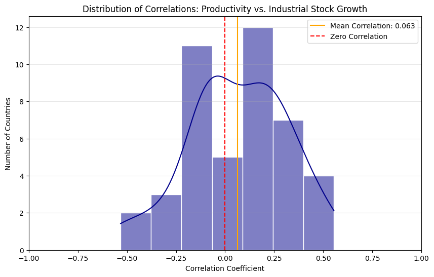
Distributions of Correlations: Stock Growth vs Industrial Stock Growth
”Distributions
Source: ECB data.

The core of this myth is the macroeconomic assumption that a more efficient workforce naturally results in a more valuable stock market. This myth has been debunked on numerous occasions(1) (2), but the disruption created by AI creates new challenges that have to be addressed. To test this, I conducted an extensive analysis on the correlation between labor productivity and stock market returns across European Union countries. The results were startling. The correlation value was only 0.063.

The 0.063 Reality Check

In the world of statistics, a correlation of 0.063 is effectively zero. This figure reveals a profound “missing link” in our economic understanding. For decades, workers in the EU became more efficient and had almost no direct impact on the country’s stock market performance.

In conducting this study, I took the data for the EU member states starting from 2005 until 2025. This time-lapse represents the period following the “.com bubble” and the beginning of the mass adoption of informational systems by many companies. As the cost of owning, operating, and managing these systems became more accessible, it represented a fresh start.

Productivity Trend
Productivity Trend
Source: ECB data.

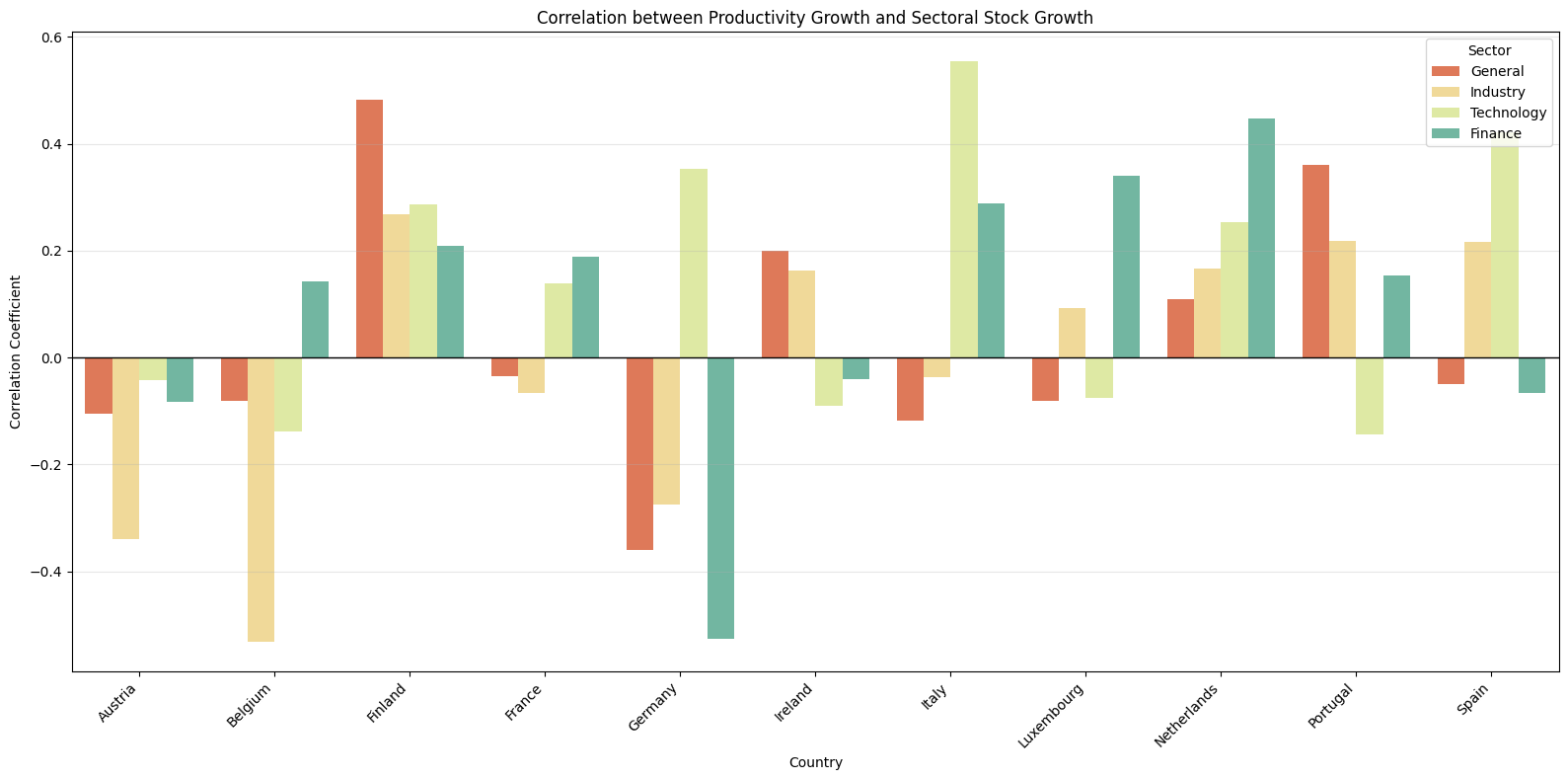
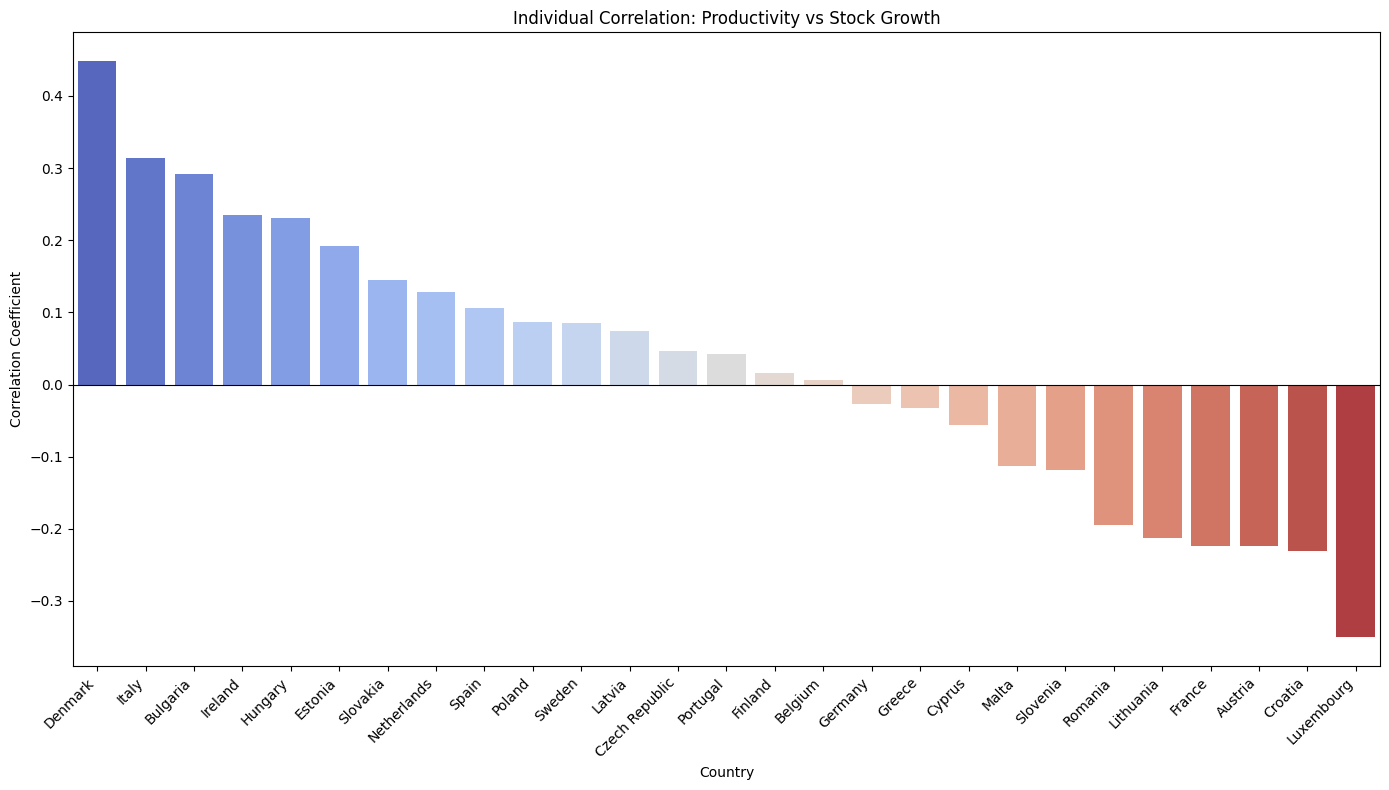
By computing the productivity with the return on the EURO STOXX, a clear result can be seen: working harder is not making the enterprise more valuable if everyone is capable of implementing similar strategies. At an individual level, some countries can excel in the implementation if the governance facilitates the projection of technology by liberating and promoting innovation. Some good examples would be the Netherlands, a leader in innovation in the technology and information sector, benefiting heavily from the adoption of the internet and outsourcing, and Italy, a counter-example in productivity growth with similarly low growth in the stock market.

Sectoral Correlation
Sectoral Productivity
Source: ECB data.

Although many countries exhibit a significant correlation between growth and productivity, the reality shows that some sectors are driving the general growth. The benefits of the new technologies implemented in the information sector led to a process simplification, reducing the due diligence and accelerating the globalization of the product and market access. While some sectors directly benefited from the implementation of the internet in the processes, the industrial process lagged in showing a similar impact from the internet adoption.

The implementation of the internet resulted in winners and losers, affecting individual companies differently and consolidating the position of global leaders in the industry. Following the .com bubble, many companies disappeared or were acquired by the companies that successfully bypassed the fast-paced changes of the new demands of the customers that encountered a truly global world for the first time (3).

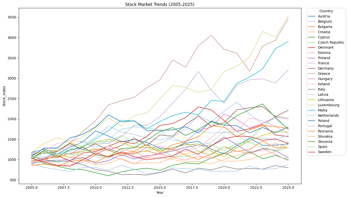
Stock Market Trends
Stock Market Trends
Source: ECB data.

This finding is the “missing link” for the AI Productivity Myth. If thirty years of digital and industrial evolution failed to bridge this gap, investors must ask why AI will be the exception and close the gap. My research suggests that productivity is a measure of how hard an economy works, whereas stock growth is a measure of how much of that work shareholders actually get to keep. In the EU, these two variables operate in parallel universes and vary vastly from one country to another.

Individual Correlation: Productivity vs Stock Growth
Stock Market Trends
Source: ECB data.

Echoes of the Internet Boom

In the late 1990s, the Internet was the “disruptive power” that promised a new era of high profits from internet sales, showing positive sentiment in the new technology (4). Specialists discussed the exponential implementation of the internet and how all companies will use it in maximizing their profits and directly impacting the prices of the stocks. Many investors were unaware of the risk involved in the investments in new technologies, and focused solely on the possible returns from their investments. The promise was very similar to the AI’s, the internet will revolutionize the world, creating a massive leap in how we exchange information.

Although the information travelled faster and everyone was benefiting from the effects of a “smaller world”, it backfired. While the technology succeeded, the investments often failed. When the bubble burst in 2000, it wasn’t because the internet stopped working; it was because the market momentum had far outpaced the actual ability of companies to turn that efficiency into profit.

Today, AI is facing the same exaggerated expectations. Investors are paying premium prices for the hope of future productivity, but they are ignoring thehardships of the adoption gap: the period where companies spend billions on Graphic Processing Units(GPU), the core of the AI systems, and energy without seeing a single cent of increased margin. This gold rush after the current stock of GPUs is leading to a speculative movement over their importance and short product cycles, leading to slow amortizations for ⅚ years, while in reality they become obsolete in ⅔ years(5).

The “Blurriness” of AI Returns

The “blurriness” of Large Language Models (LLMs) refers to the difficulty in measuring their return on investment (ROI). The investment in AI chips, developing agents, and managing data centers comes into effect without prior benchmarks on how such investments should be estimated, and it is hard to quantify their success in monetary terms or advantages against the competitors. Unlike a new factory machine that produces 10% more widgets, an LLM’s impact on knowledge and streamlining is harder to capture on a balance sheet.

  • The CapEx Trap: Companies are engaged in an “Arms Race,” spending record amounts on infrastructure. Firms are paying considerable amounts on implementation costs (licensing, retraining, power, cloud, cybersecurity,etc.), but often eats up the savings the AI was supposed to generate.
  • The Perfect Competition Paradox: If every firm uses AI to work 50% faster, no single firm has a competitive advantage. Competition forces them to lower prices, passing the productivity gain to the consumer while the investor is left with higher tech costs and lower retention of both earnings and customers.
  • Front-Running the Gains: The stock market is forward-looking. Most expected gains are already baked into today’s prices. When a company finally reports a “good” productivity increase, the stock may drop because it wasn’t the “miraculous” increase the market demanded to justify its valuation.

Conclusion: Why the Low Correlation Matters

The key takeaway is the danger of the 0.063 correlation. It proves that efficiency is the tool for survival, but not a guaranteed engine for wealth. In the European Union (EU), efficiency gains are frequently absorbed by regulatory compliance, labor costs, and competitive pricing before they ever reach the bottom line.

Why should I be interested in this post?

As we move through 2026, the “blurriness” of AI will likely resolve into a clear picture of high costs and incremental gains. For everyone, the lesson should be clear: do not mistake a technological revolution for a guaranteed stock market return. In an environment where the correlation between productivity and returns is as low, the “AI Myth” is a luxury that few can afford to believe in.

Other SimTrader Blogs:

   ▶ Mahé FERRET Behavioral Finance

References

(1) Chun, H., Kim, J. W., & Morck, R. (2016). Productivity growth and stock returns: firm-and aggregate-level analyses. Applied Economics, 48(38), 3644-3664.

(2) Pellegrini, C. B., Romelli, D., & Sironi, E. (2011). The impact of governance and productivity on stock returns in European industrial companies. Investment management and financial innovations, (8, Iss. 4), 20-28.

(3) Johansen, A., & Sornette, D. (2000). The Nasdaq crash of April 2000: Yet another example of log-periodicity in a speculative bubble ending in a crash. The European Physical Journal B-Condensed Matter and Complex Systems, 17(2), 319-328.

(4) Bandyopadhyay, S., Lin, G., & Zhang, Y. (2001). A critical review of pricing strategies for online business models.

(5) Lifespan of AI chips- the 300 billion question

Data sources:

European Central Bank EURO STOXX

European Central Bank~Productivity Growth

MSCI Report

About the author

The article was written in January 2026 by Andrei DONTU (ESSEC Business School, Global Bachelor in Business Administration (GBBA), 2025-2026).

   ▶ Read all posts written by Andrei DONTU

“The big money is not in the buying and selling, but in the waiting.” – Charlie Munger

In an era dominated by instant trading for individuals, high-frequency trading firms, ever-faster market infrastructures, and social-media-driven market narratives, patience has become an underrated virtue.

Hadrien PUCHE

In this article, Hadrien PUCHE (ESSEC Business School, Grande École Program, Master in Management, 2023-2027) comments on Charlie Munger’s famous quote about the role of patience and discipline in long-term investing, and what it teaches us about the power of compounding, temperament, and time.

About Charlie Munger

Charlie Munger (1924–2023) was the long-time vice chairman of Berkshire Hathaway, and Warren Buffett’s closest business partner for over 50 years. Munger profoundly influenced Buffett’s philosophy, steering him toward buying high-quality businesses and holding them for the long run.

Munger’s wisdom combined principles from psychology, economics, and philosophy to form a timeless view of markets and human behavior.

Charlie Munger
Source: Wikimedia Commons

About the quote

“The big money is not in the buying and selling, but in the waiting.”

This quote is one of Charlie Munger’s most enduring lessons, though its origins date back to the 1923 classic Reminiscences of a Stock Operator by Jesse Livermore. Munger adopted and popularized this wisdom throughout his career, most notably during the Berkshire Hathaway annual shareholder meetings, to explain the firm’s extraordinary success.

The quote encapsulates the essence of long-term investing: wealth is not built through frequent market timing, but through the quiet power of patience and compounding. Munger and Buffett repeatedly emphasized that the most successful investors are not those who move the fastest, but those who possess the “temperament” to sit still when the rest of the market is acting impulsively.

Ultimately, this principle suggests that time, rather than timing, is the real driver of wealth creation. In Munger’s view, “waiting” is an active strategy. It is the disciplined choice to let your initial thesis play out without the interference of market noise or emotional reactions.

Analysis of the quote

This quote highlights a key principle of investing: activity is not the same as value creation. Many investors confuse motion with progress, feeling the urge to trade constantly in response to news, trends, or short-term price fluctuations.

Munger’s philosophy reminds us that wealth is not “generated” by the act of trading; it is accumulated by letting compounding do its work, a process that rewards patience and conviction far more than speed. Charlie Munger’s observation, “The first rule of compounding is to never interrupt it unnecessarily,” distills decades of investing wisdom into a single principle: long-term wealth creation depends less on brilliance than on consistency and emotional endurance.

Every time an investor exits a position due to short-term fear or a desire to “lock in” small gains, they “reset” the clock and sacrifice the exponential growth that occurs in the final years of a holding period. Furthermore, frequent activity creates “leakage” through trading costs and taxes, which act as a constant drag on returns.

In essence, Munger’s rule is a call for consistency over cleverness, emphasizing that compounding rewards time and temperament, qualities far rarer and more valuable than momentary flashes of insight.

Financial concepts related to the quote

I present below three financial concepts: the power of compounding, opportunity cost and value of inactivity, and the patience premium of investor behavior.

The Power of Compounding

Compounding is the process by which returns themselves begin to generate further returns: a self-reinforcing cycle of growth. Its effect is exponential rather than linear: small, steady gains, that accumulate dramatically over time.

For instance, at a 10% annual return, an investment of 100 grows to 110 after one year, 259 after ten years, and 1,745 after thirty years. The formula for the future value Vf is:

Vf = Vi × (1 + ρ / n)n × t

Where ρ (rho) is the interest rate and n is the number of times that interest is compounded every year. The key variable is time (t): the longer the compounding process continues uninterrupted, the greater the growth. Interruptions through withdrawals or frequent trading can significantly reduce the ultimate value of the investment.

Opportunity Cost and the value of inactivity

In behavioral and financial terms, opportunity cost is what one sacrifices by choosing one action over another. Many investors mistakenly equate activity with progress, yet frequent transactions often lead to higher costs, taxes, and emotional errors. As Buffett and Munger emphasize, strategic inactivity (allowing quality investments to compound) is often the most effective decision one can make.

The “Goalkeeper Syndrome”: A Lesson from the Pitch

This tendency to favor motion over stillness is driven by action bias. A study by Bar-Eli et al. (2007) on elite soccer goalkeepers found that while goalkeepers have the highest probability of stopping a penalty by staying in the center of the goal, they only do so 6.3% of the time. In over 93% of cases, they dive to the left or right.

This “Goalkeeper Syndrome” is best explained by Daniel Kahneman’s Norm Theory (Thinking, Fast and Slow, 2011). Kahneman demonstrates that humans feel more intense regret when a bad outcome results from an action than from an inaction—unless the action is the norm.

In the goalkeeper’s case, jumping is the social norm. If a goal is scored while the keeper stands still, they appear to have “done nothing,” which is socially and emotionally harder to bear. If they dive and miss, they have “tried.” For investors, this creates a dangerous paradox. In the investment industry, “activity” is often the norm. A fund manager who does nothing during a market shift risks being seen as lazy or incompetent. By “diving” into a new trade, they protect themselves from the intense regret of being wrong while being inactive.

Recognizing this bias is essential for any finance professional. True discipline lies in knowing when to act, and having the courage to stay in the center of the net when everyone else is jumping.

The Patience Premium and Investor Behavior

Behavioral finance demonstrates that human psychology often works against long-term success. Biases like overconfidence, loss aversion, and herd behavior push investors to buy high and sell low. The ability to stay rational when others panic — to maintain conviction in one’s analysis rather than react to market noise — creates a powerful advantage.

This discipline produces what can be called a patience premium: higher long-term returns earned simply by avoiding costly mistakes. As Warren Buffett summarized, “The stock market is a device for transferring money from the impatient to the patient.”

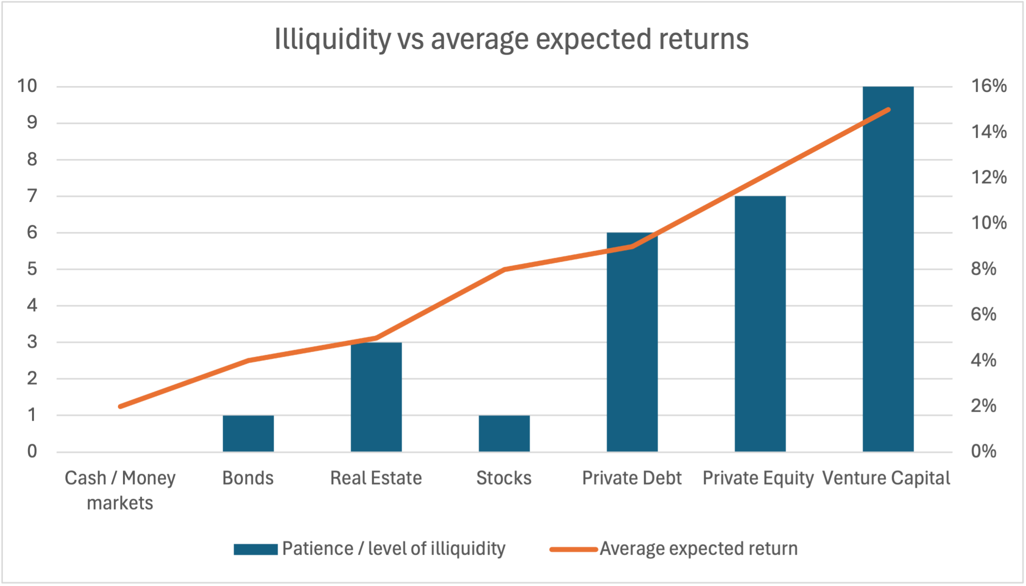
Private equity provides a practical illustration of the patience premium. Investments in private companies are typically illiquid for many years, forcing investors to maintain a long-term perspective. This “forced patience” comes with a reward: private equity funds historically deliver higher returns than public markets, reflecting both the illiquidity premium and the benefits of disciplined, long-term value creation.

Illiquidity vs average expected returns graph
In general, more illiquid investments offer higher expected returns, as investors are compensated for the additional illiquidity risk. Note: Values are illustrative.

Beyond the financial premium, illiquidity serves as a vital behavioral guardrail. In public markets, the ability to sell an asset instantly makes it far easier to succumb to panic during market turbulence. You cannot “panic sell” an asset that you cannot sell quickly. By removing the option for impulsive exits, illiquid structures protect investors from their own emotional reactions, ensuring that compounding is never interrupted unnecessarily.

My opinion about this quote

I believe this quote captures one of the hardest truths in investing: sometimes the most profitable action is to do nothing. In today’s world of trading apps, meme stocks, and 24-hour market news, patience feels almost countercultural. Investors are constantly nudged to act, reacting to every headline or social media hype. Yet, this very activity often erodes long-term returns.

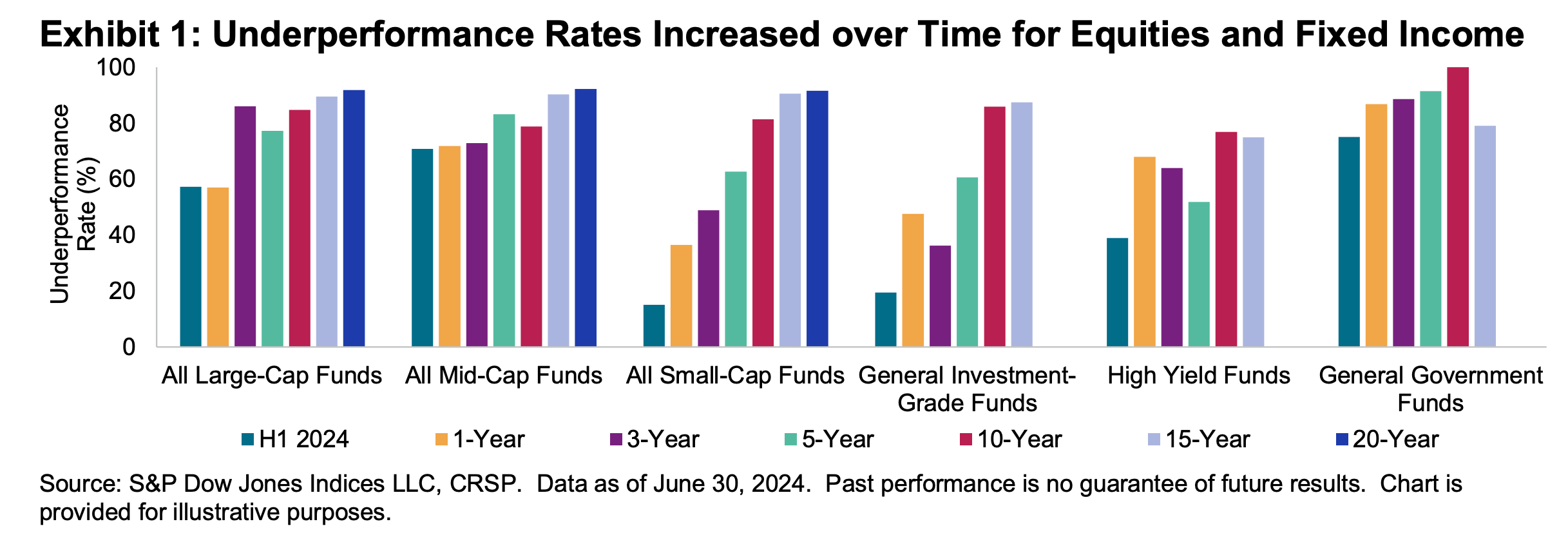
One concrete way to see this principle in action is through passive investing. Actively managed funds exist with the goal of outperforming their benchmark indexes, yet studies like SPIVA (S&P Indices Versus Active) show that most fail to do so over long periods. For instance, over 10-year periods, roughly 80% of U.S. equity funds underperformed the S&P 500 index.

underperformance rates over time SPIVA
This SPIVA graph illustrates that most actively managed funds underperform their benchmark index over the long term, highlighting the advantage of passive investing.

However, this debate between active and passive management leads us to a fascinating theoretical tension: the Grossman-Stiglitz Paradox. If every investor followed the “sweet fruit” of passive investing because it is statistically superior, the market would cease to function properly and make active investment worth it again.

The paradox, formulated by Sanford Grossman and Joseph Stiglitz in 1980, suggests that markets cannot be perfectly efficient. If a market were perfectly efficient (meaning all information is already reflected in the price), no one would have an incentive to spend time uncovering new information. But if no one uncovers information, the market becomes inefficient. Therefore, the market must remain “efficiently inefficient”: it requires active managers to do the “bitter” work of research, even if they often fail to beat the index, so that passive investors can enjoy the “sweet” ride of a mostly accurate market price.

Yet, the lesson is clear: staying invested in a broadly diversified index often beats trying to “time” the market. The patient investor harnesses compounding without the friction of trading costs, taxes, and emotional mistakes. As Munger famously noted, “the big money is not in the buying and selling, but in the waiting.” It’s not about inactivity for its own sake; it’s about informed, disciplined inactivity.

Why should you be interested in this post?

Beyond investing, this quote is about cultivating a mindset of patience, discipline and rational thinking that can separate successful individuals from the crowd. Mastering the art of waiting will give you an edge, no matter which industry you desire to work in.

Careers, skills, and personal growth all compound like investments; building expertise takes time. Quick wins may feel gratifying, but long-term impact comes to those who embrace patience and persist through the quiet, unglamorous work that others sometimes avoid.

Related posts

   ▶ All posts about Quotes

   ▶ Hadrien PUCHE “The stock market is filled with individuals who know the price of everything, but the value of nothing.” – Philip Fisher.

   ▶ Hadrien PUCHE “Most people overestimate what they can do in a year and underestimate what they can do in ten.” – Bill Gates

   ▶ Hadrien PUCHE “Patience is bitter, but its fruit is sweet.” – Aristotle

Useful resources

Berkshire Hathaway’s website: www.berkshirehathaway.com

Munger, Charlie. Poor Charlie’s Almanack, 2005.

Buffett, Warren. Berkshire Hathaway Shareholder Letters.

Kahneman, Daniel. Thinking, Fast and Slow, 2011. (especially Chapter 32 on regret and norm theory).

Bar-Eli, M., Azar, O. H., Ritov, I., Keidar-Levin, Y., & Schein, G. (2007) Action bias among elite soccer goalkeepers: The case of penalty kicks. Journal of Economic Psychology, 28(5), 606-621.

About the Author

This article was written in January 2026 by Hadrien PUCHE (ESSEC Business School, Grande École Program, Master in Management, 2023-2027).

   ▶ Read all posts written by Hadrien PUCHE

Patience is bitter, but its fruit is sweet – Aristotle

Waiting is never easy. In life, at work, and certainly in finance, we are naturally drawn to quick outcomes and instant gratification. This preference for immediacy is built into our psychology, a leftover from a time when obtaining resources in the present meant survival.

This is why the quote resonates so strongly. It expresses a universal tension between the comfort of the present and the rewards that arrive only through the passage of time. The analogy with food captures the idea beautifully: most of us choose what tastes good now, such as a sugary treat or a risky trade, instead of what will benefit us later, like a healthy meal or a disciplined investment. Markets consistently reward discipline, yet human nature urges us toward the immediate emotional release provided by action.

Hadrien PUCHE

In this article, Hadrien PUCHE (ESSEC, Grande École Program, Master in Management, 2023-2027) comments on Aristotle’s famous quote about the discipline required for long-term success.

Aristotle

Aristotle
Source: Wikimedia Commons

Aristotle was one of the most influential thinkers in ancient Greece and a foundational figure of Western philosophy. Born in the fourth century BCE in Stagira, he studied under Plato and later tutored Alexander the Great. He founded the Lyceum, emphasizing careful observation and reason across logic, ethics, and metaphysics.

In ethics, Aristotle focused on character development through deliberate practice. He believed virtues like patience are not natural gifts, but habits formed through repeated disciplined actions. This connects directly with long-term investing, which rewards consistent behaviors and emotional mastery. While the quote is often misattributed, its message stands at the center of successful investing: the true test is not intelligence, but emotional endurance.

Analysis of the Quote

This quote encompasses the central tension in investing: the difficulty of the present versus the reward of the future. In markets, patience is an active discipline. It requires staying invested through volatility and resisting popular trends. These moments of discomfort represent the “bitter” side of patience.

The “sweet fruit” is compounding—a force that transforms small, consistent gains into extraordinary outcomes. It only rewards those who give it time. Legendary investors like Buffett, Lynch, and Munger insist that patience, not genius, accounts for their success. The investor who endures temporary discomfort for long-term clarity exercises patience exactly as Aristotle would have understood it.

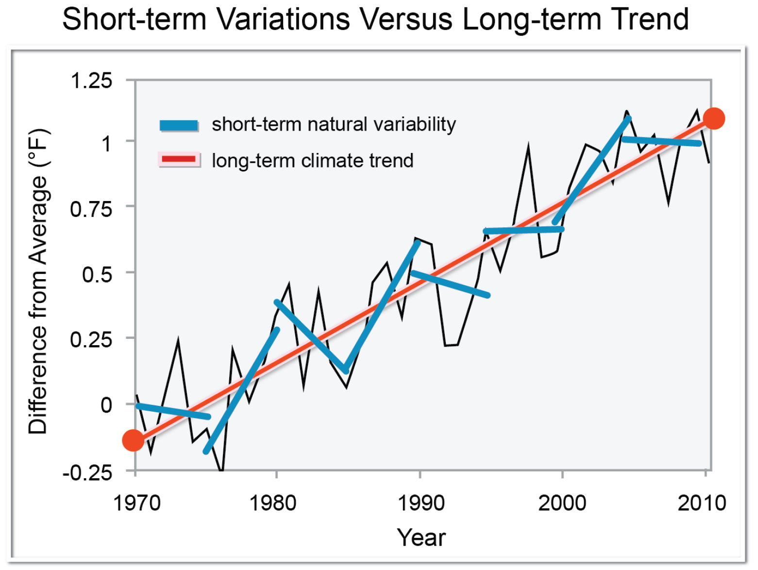
Short term vs long term trends
Short-term variations matter less than the long-term average trend. Source: Wikimedia Commons.

Historical Failures of Patience

History shows that impatience fueled many financial catastrophes. During the 17th-century **Tulip Mania**, prices soared as traders flipped bulbs for quick profits, only to see the market collapse in days. The same pattern repeated in the **South Sea Bubble** and the **Dot-Com Bubble**, where speculation displaced fundamentals. Across these episodes, short-term excitement overshadowed long-term thinking, turning promising opportunities into costly lessons.

Financial Concepts Tied to the Quote

Time Horizon: The Power of μ over σ

Having a long time horizon allows investors to rely on fundamentals rather than hype. Quantitatively, this is the battle between the expected return ($\mu$) and volatility ($\sigma$). While market prices are dominated by $\sigma$ (random swings) in the short term, the long-term outcome is driven by $\mu$ (intrinsic growth).

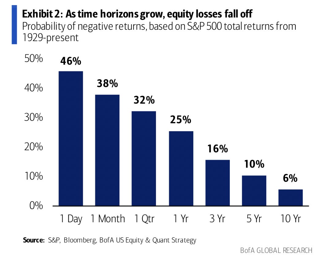
Probability of loss depending on time

Viewing decisions through a 10 or 20-year perspective reframes downturns as opportunities. This is due to time diversification: as the holding period ($t$) expands, the annualized volatility decreases at a rate of $1/\sqrt{t}$. Time reduces the “noise,” making the fundamental $\mu$ eventually overwhelm the temporary $\sigma$.

Risk and Reward Balance

Patience does not remove risk, but it improves emotional endurance. Impatient investors often understand risk in theory but panic when it appears on a statement, leading to selling at the worst time. Patient investors focus on long-term goals, allowing time to work as a risk management tool.

Opportunity Cost and the Value of Inactivity

In behavioral finance, opportunity cost is what one sacrifices by choosing one action over another. Many investors mistakenly equate activity with progress, yet frequent transactions lead to higher costs and taxes. Buffett and Munger emphasize that strategic inactivity is often the most effective decision.

This tendency to favor motion is driven by action bias, or the “Goalkeeper Syndrome.” A study by Bar-Eli et al. (2007) found that goalkeepers have the highest probability of stopping a penalty by staying in the center of the goal, yet they do so only 6.3% of the time. They dive because the regret of “doing nothing” feels worse than the regret of a failed action. This carries over to investment management, where investors churn portfolios during volatility just to feel in control.

My Opinion in a Modern Context

This quote is especially relevant today. Trading apps encourage activity, and social media amplifies FOMO (Fear of Missing Out). In this environment, patience is a competitive advantage. Successful investors are often not the smartest, but the most consistent. In a world that rewards speed, the courage to wait becomes rare and extremely valuable.

Why This Quote Should Matter to You

Patience isn’t just a pleasant virtue; it’s a tool that shapes results. Whether building a career or managing finances, patience allows you to:

  • Make thoughtful choices grounded in clarity rather than impulse.
  • Avoid stress-driven errors.
  • Stay aligned with long-term goals despite short-term distractions.

Related Posts on the SimTrade Blog

   ▶ All posts about Quotes

   ▶ Hadrien PUCHE “Most people overestimate what they can do in a year…” – Bill Gates

   ▶ Hadrien PUCHE “Price is what you pay, value is what you get” – Warren Buffett

Useful resources

Aristotle. Nicomachean Ethics. Translated by Terence Irwin. Hackett Publishing, 1999.

Bar-Eli, M., Azar, O. H., Ritov, I., Keidar-Levin, Y., & Schein, G. (2007). Action bias among elite soccer goalkeepers: The case of penalty kicks. Journal of Economic Psychology, 28(5), 606-621.

Kindleberger, Charles P., and Robert Aliber. Manias, Panics, and Crashes. Palgrave Macmillan, 2011.

Mackay, Charles. Extraordinary Popular Delusions and the Madness of Crowds. Wordsworth Editions, 1995.

About the Author

The article was written in January 2026 by Hadrien PUCHE (ESSEC, Grande École Program, Master in Management – 2023-2027).

Modeling Asset Prices in Financial Markets: Arithmetic and Geometric Brownian Motions

Saral BINDAL

In this article, Saral BINDAL (Indian Institute of Technology Kharagpur, Metallurgical and Materials Engineering, 2024-2028 & Research assistant at ESSEC Business School) presents two statistical models used in finance to describe the time behavior of asset prices: the arithmetic Brownian motion (ABM) and the geometric Brownian motion (GBM).

Introduction

In financial markets, performance over time is governed by three fundamental variables: the drift (μ), volatility (σ), and maybe most importantly time (T). The drift represents the expected growth rate of the price and corresponds to the expected return of assets or portfolios. Volatility measures the uncertainty or risk associated with price fluctuations around this expected growth and corresponds to the standard deviation of returns. The relationship between these variables reflects the trade-off between risk and return. Time, which is related to the investment horizon set by the investor, determines how both performance and risk accumulate. Together, these variables form the foundation of asset pricing to model the behavior of market price over time, and in fine the performance of the investor at their investment horizon.

Modeling asset prices

Asset price modeling is used to understand the expected return and risk in asset management, risk management, and the pricing of complex financial products such as options and structured products. Although asset prices are influenced by countless unpredictable risk factors, quants in finance always try to find a parsimonious way to model asset prices (using a few parameters only).

The first study of asset price modelling dates from Louis Bachelier in 1900, in his doctoral thesis Théorie de la Spéculation (The Theory of Speculation), where he modelled stock prices as a random walk and applied this framework to option valuation. Later, in 1923, the mathematician Norbert Wiener formalized these ideas as the Wiener process, providing the rigorous stochastic foundation that underpins modern finance.

In the 1960s, Paul Samuelson refined Bachelier’s model by introducing the geometric Brownian motion, which ensures positive stock prices following a lognormal statistical distribution. His 1965 paper “Rational Theory of Warrant Pricing” laid the groundwork for modern asset price modelling, showing that discounted stock prices follow a martingale.

We detail below the two models usually used in finance to model the evolution of asset prices over time: the arithmetic Brownian motion (ABM) and the geometric Brownian motion (GBM). We will then use these models to simulate the evolution of asset prices over time with the Monte Carlo simulation method.

Arithmetic Brownian motion (ABM)

Theory

One of the most widely used stochastic processes in financial modeling is the arithmetic Brownian motion, also known as the Wiener process. It is a continuous stochastic process with normally distributed increments. Using the Wiener process notation, an asset price model in continuous time based on an ABM can be expressed as the following stochastic differential equation (SDE):


SDE for the arithmetic Brownian motion

where:

  • dSt = infinitesimal change in asset price at time t t
  • μ = drift (growth rate of the asset price)
  • σ = volatility (standard deviation)
  • dWt = infinitesimal increment of wiener process (N(0,dt))

Note that the standard Brownian motion is a special case of the arithmetic Brownian motion with a mean equal to zero and a variance equal to one.

In this model, both μ and σ are assumed to be constant over time. It can be shown that the probability distribution function of the future price is a normal distribution implying a strictly positive (although negligible in most cases) probability for the price to be negative.

Integrating the SDE for dSt over a finite interval (from time 0 to time t), we get:


Integrated SDE for the arithmetic Brownian motion

Here, Wt is defined as Wt = √t · Zt, where Zt is a normal random variable drawn from the standard distribution N(0, 1) with mean equal to 0 and variance equal to 1.

At any date t, we can also compute the expected value and a confidence interval such that the asset price St lies between the lower and upper bound of the interval with probability equal to 1-α.


Theoritical formulas for mean, upper and lower limits of ABM model

Where S0 is the initial asset price and zα.

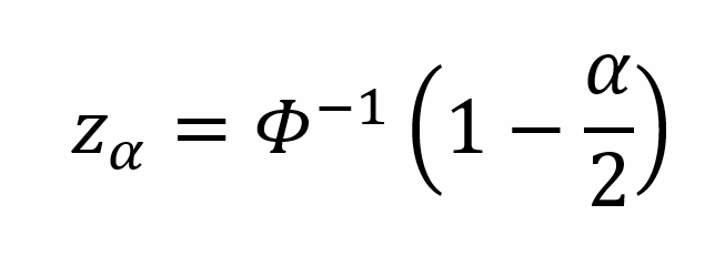
The z-score for a confidence level of (1 – α) can be calculated as:


z-score formula

where Φ-1 denotes the inverse cumulative distribution function (CDF) of the standard normal distribution.

For example the statistical z-score (zα) values for 66%, 95%, and 99% confidence intervals are as the following:


z-score examples

Monte Carlo simulations with ABM

Since Monte Carlo simulations are performed in discrete time, the underlying continuous-time asset price process (ABM) is approximated using the Euler–Maruyama discretization of SDEs (see Maruyama, 1955), as shown below.


Discretization formula for the arithmetic Brownian motion (ABM)

where Δt denotes the time step, expressed in the same time units as the drift parameter μ and the volatility parameter σ (usually the annual unit). For example, Δt may be equal to one day (=1/252) or one month (=1/12).

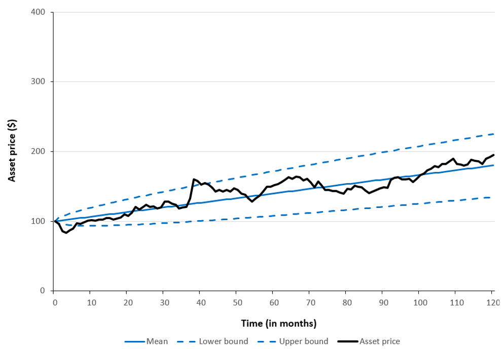
Figure 1 below illustrates a single simulated asset price path under an arithmetic Brownian motion (ABM), sampled at monthly intervals (Δt = 1/12) over a 10-year horizon (T = 10). Alongside the simulated path, the figure shows the expected (mean) price trajectory and the corresponding upper and lower bounds of a 66% confidence interval. In this example, the model assumes an annual drift (μ) of $8, representing the expected growth rate, and an annual volatility (σ) of $15, capturing random price fluctuations. The initial asset price (S0) is equal to $100.

Figure 1. Single Monte Carlo–simulated asset price path under an Arithmetic Brownian Motion model.
A Monte Carlo–simulated price path under an arithmetic Brownian motion model
Source: computation by the author (with Excel).

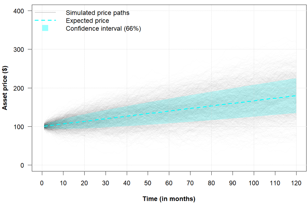
Figure 2 below illustrates 1,000 simulated asset price paths generated under an arithmetic Brownian motion (ABM). In addition to the simulated paths, the figure displays the expected (mean) price trajectory along with the corresponding upper and lower bounds of a 66% confidence interval, using the same parameter settings as in Figure 1.

Figure 2. Monte Carlo–simulated asset price paths under an Arithmetic Brownian Motion model.
Monte Carlo–simulated price paths under an arithmetic Brownian motion model.
Source: computation by the author (with R).

Geometric Brownian motion (GBM)

Theory

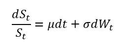
Since an arithmetic Brownian motion (ABM) can take negative values, it is unsuitable for directly modeling stock prices if we assume limited liability for investors. Under limited liability, an investor’s maximum possible loss is indeed confined to their initial investment, implying that asset prices cannot fall below zero. To address this limitation, financial models instead use geometric Brownian motion (GBM), a non-negative stochastic process that is widely employed to describe the evolution of asset prices. Using the Wiener process notation, an asset price model in continuous time based on a GBM can be expressed as the following stochastic differential equation (SDE):


SDE for the geometric Brownian motion (GBM)

where:

  • St = asset price at time t t
  • μ = drift (growth rate of the asset price)
  • σ = volatility (standard deviation)
  • dWt = infinitesimal increment of wiener process (N(0,dt))

Integrating the SDE for dSt/St over a finite interval, we get:


Integrated SDE for the geometric Brownian motion (GBM)

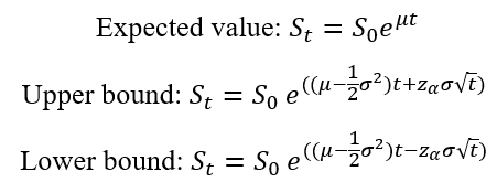
The theoretical expected value and confidence intervals are given analytically by the following expressions:


Theoritical formulas for mean, upper and lower limits of GBM model

Monte Carlo simulations with GBM

To implement Monte Carlo simulations, we approximate the underlying continuous-time process in discrete time, yielding:


Asset price under discrete GBM

where Zt is a standard normal random variable drawn from the distribution N(0, 1) and Δt denotes the time step, chosen so that it is expressed in the same time units as the drift parameter μ and the volatility parameter σ.

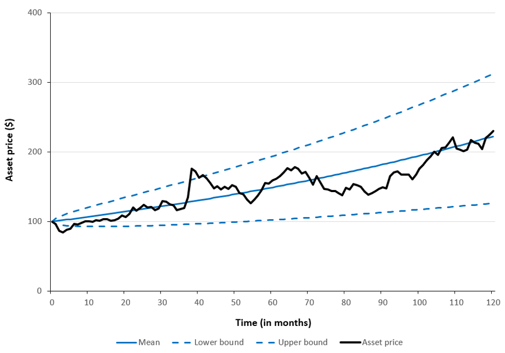
Figure 3 below illustrates a single simulated asset price path under a geometric Brownian motion (GBM), sampled at monthly intervals (Δt = 1/12) over a 10-year horizon (T = 10). Alongside the simulated path, the figure shows the expected (mean) price trajectory and the corresponding upper and lower bounds of a 66% confidence interval. In this example, the model assumes an annual drift (μ) of 8%, representing the expected growth rate, and an annual volatility (σ) of 15%, capturing random price fluctuations. The initial asset price is S0 €100.

Figure 3. Monte Carlo–simulated asset price path under a Geometric Brownian Motion model.
Monte Carlo–simulated asset price path under a GBM model.
Source: computation by the author (with Excel).

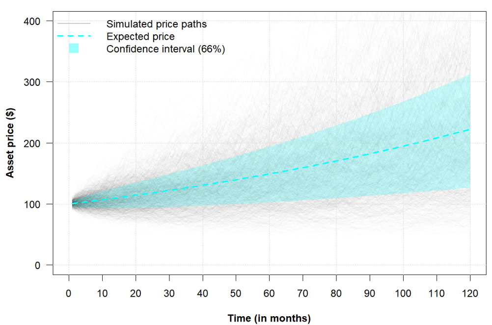
Figure 4 below illustrates 1,000 simulated asset price paths generated under a geometric Brownian motion (GBM). In addition to the simulated paths, the figure displays the expected (mean) price trajectory along with the corresponding upper and lower bounds of a 66% confidence interval, using the same parameter settings as in Figure 3.

Figure 4. Monte Carlo–simulated asset price paths under a Standard Brownian Motion model.
 Monte Carlo–simulated asset price paths under a Geometric Brownian Motion model.
Source: computation by the author (with R).

Discussion

The drift μ represents the expected rate of growth of asset prices, so its cumulative contribution increases linearly with time as μT. In contrast, volatility σ captures investment risk, and its cumulative impact scales with the square root of time as σ√T. As a result, over short horizons stochastic shocks tend to dominate the deterministic drift, whereas over longer horizons the expected growth component becomes increasingly prominent.

When many paths for the asset price are simulated and plotted over time, the resulting trajectories form a cone-shaped region, commonly referred to as a fan chart. The center of this fan traces the smooth expected path governed by the drift μ, while the widening envelope reflects the growing dispersion of outcomes induced by volatility σ.

This representation underscores a key implication for long-term investing and risk management: uncertainty expands with the investment horizon even when model parameters remain constant. While the expected value evolves predictably and linearly through time, the range of plausible outcomes broadens at a slower, square-root rate, shaping the risk–return trade-off across different time scales.

You can download the Excel file provided below for generating Monte Carlo Simulations for asset prices modeled on arithmetic and geometric Brownian motion.

Download the Excel file.

You can download the Python code provided below, for generating Monte Carlo Simulations for asset prices modeled on arithmetic and geometric Brownian motion.

Download the Python code.

Alternatively, you can download the R code below with the same functionality as in the Python file.

 Download the R code.

Link between the ABM and the GBM

The ABM and GBM models are fundamentally different: the drift for the ABM is additive while the drift for the GBM is multiplicative. Moreover, the statistical distribution for the price for the ABM is a normal distribution while the statistical distribution for the GBM is a log-normal distribution. However, we can study the relationship between the two models as they are both used to model the same phenomenon, the evolution of asset prices over time in our case.

We can especially study the relationship between the two parameters of the two models, μ and σ. In the presentation above, we used the same notations for μ and σ for the two models, but the values of these parameters for the two models will be different when we apply these models to the same phenomenon. There is no mapping of the ABM and GBM in the price space such that we get the same results as the two models are fundamentally different.

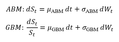
Let us rewrite the two models (in terms of SDE) by differentiating the parameters for each model:


SDE for the ABM and GBM

To model the same phenomenon, we can use the following relationship between the parameters of the ABM and GBM models:


Link between the ABM and GBM parameters.

To make the two models comparable in terms of price behavior, an ABM can locally approximate GBM by matching instantaneous drift and volatility such that:


Local link between the ABM and GBM parameters.

This local correspondence is state-dependent and time-varying, and therefore not a true parameter equivalence.

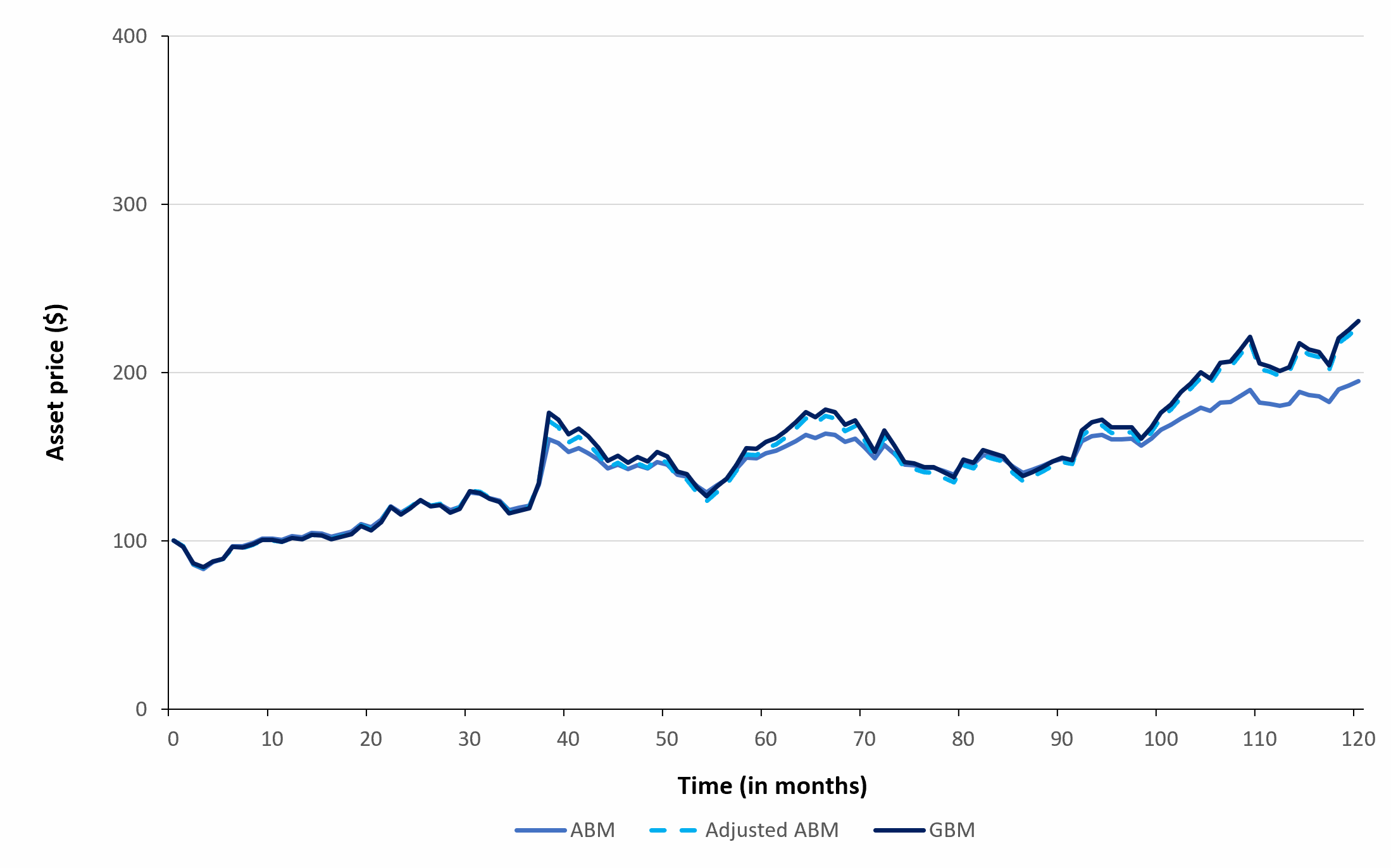
Figure 5 below compares the asset price path for an ABM, monthly adjusted ABM and a GBM.


Simulated asset price paths for ABM, adjusted ABM and GBM.

Why should I be interested in this post?

Understanding how asset prices are modeled, and in particular the difference between additive and multiplicative price dynamics, is essential for building strong intuition about how prices evolve over time under uncertainty. This understanding forms the foundation of modern risk management, as it directly informs concepts such as capital protection, downside risk, and the long-term behavior of investment portfolios.

Related posts on the SimTrade blog

   ▶ Saral BINDAL Historical Volatility

   ▶ Saral BINDAL Implied Volatility and Option Prices

   ▶ Jayati WALIA Brownian Motion in Finance

   ▶ Jayati WALIA Monte Carlo simulation method

Useful resources

Academic research

Bachelier L. (1900) Théorie de la spéculation. Annales scientifiques de l’École Normale Supérieure, 3e série, 17, 21–86.

Kataoka S. (1963) A stochastic programming model. Econometrica, 31, 181–196.

Lawler G.F. (2006) Introduction to Stochastic Processes, 2nd Edition, Chapman & Hall/CRC, Chapter “Brownian Motion”, 201–224.

Maruyama G. (1955) Continuous Markov processes and stochastic equations. Rendiconti del Circolo Matematico di Palermo, 4, 48–90.

Samuelson P.A. (1965) Rational theory of warrant pricing. Industrial Management Review, 6(2), 13–39.

Telser L. G. (1955) Safety-first and hedging. Review of Economic Studies, 23, 1–16.

Wiener N. (1923) Differential-space. Journal of Mathematics and Physics, 2, 131–174.

Other

H. Hamedani, Brownian Motion as the Limit of a Symmetric Random Walk, ProbabilityCourse.com Online chapter section.

About the author

The article was written in January 2026 by Saral BINDAL (Indian Institute of Technology Kharagpur, Metallurgical and Materials Engineering, 2024-2028 & Research assistant at ESSEC Business School).

   ▶ Read all posts written by Saral BINDAL.

Valuation in Niche Sectors: Using Trading Comparables and Precedent Transactions When No Perfect Peers Exist

Ian DI MUZIO

In this article, Ian DI MUZIO (ESSEC Business School, Master in Finance (MiF), 2025–2027) discusses how valuation practitioners use trading comparables and precedent transactions when no truly “perfect” peers exist, and how to build a defensible valuation framework in Mergers & Acquisitions (M&A) for hybrid or niche sectors.

Context and objective

In valuation textbooks, comparable companies and precedent transactions appear straightforward: an analyst selects a sector in a database, obtains a clean peer group, computes an EV/EBITDA range, and applies it to the target. In practice, this situation is rare.

In real M&A mandates, the target often operates at the intersection of several activities (e.g. media intelligence, marketing technology, and consulting), across multiple geographies, with competitors that are mostly private or poorly disclosed.

Practitioners typically rely on databases such as Capital IQ, Refinitiv, PitchBook or Orbis. While these tools are powerful, they often return peer groups that are either too broad (mixing unrelated business models) or too narrow (excluding relevant private competitors). Private peers, even when strategically closest, usually cannot be used directly because they do not publish sufficiently detailed or standardized financial statements.

The objective of this article is therefore to provide an operational framework for valuing companies in such conditions. It explains:

  • What trading comparables and precedent transactions really measure;
  • Why “perfect” peers almost never exist in practice;
  • How to construct and clean a comps set in hybrid sectors;
  • How to use precedent transactions when listed peers are scarce;
  • How to combine these tools with discounted cash-flow (DCF) analysis and professional judgment.

The target reader is a student or junior analyst who already understands the intuition behind EV/EBITDA (enterprise value divided by earnings before interest, taxes, depreciation and amortisation), but wants to understand how experienced deal teams reason when databases do not provide obvious answers.

Trading comparables: what they measure in practice

Trading comparables rely on the idea that listed companies with similar risk, growth and operating characteristics should trade at comparable valuation multiples.

The construction of trading multiples follows three technical steps.

First, equity value is converted into enterprise value (EV):

Enterprise Value = Equity Value + Net Debt + Preferred Equity + Minority Interests – Non-operating Cash and Investments.

This adjustment ensures consistency between the numerator (EV) and the denominator (operating metrics such as EBITDA), which reflect the performance of the entire firm.

Second, the denominator is selected and cleaned. Common denominators include LTM or forward revenue, EBITDA or EBIT. EBITDA is typically adjusted to exclude non-recurring items such as restructuring costs, impairments or exceptional litigation expenses.

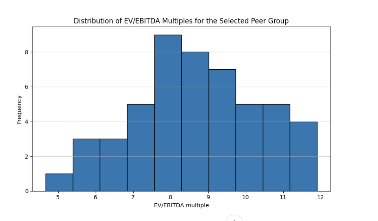
Third, analysts interpret the distribution of multiples rather than relying on a simple average. Dispersion reflects differences in growth, margins, business quality and risk. When peers are imperfect, this dispersion becomes a key analytical input.

EV/EBITDA distribution
Figure 1 – Distribution of EV/EBITDA multiples for a selected peer group in the media and marketing technology space. The figure is based on a simulated dataset constructed to mirror typical outputs from Capital IQ and Refinitiv for educational purposes. The target company is positioned within the range based on its growth, margin and risk profile.

Precedent transactions: what trading comps do not capture

Precedent transactions analyse valuation multiples paid in actual M&A deals. While computed in a similar way to trading multiples, they capture additional economic dimensions, as explained below.

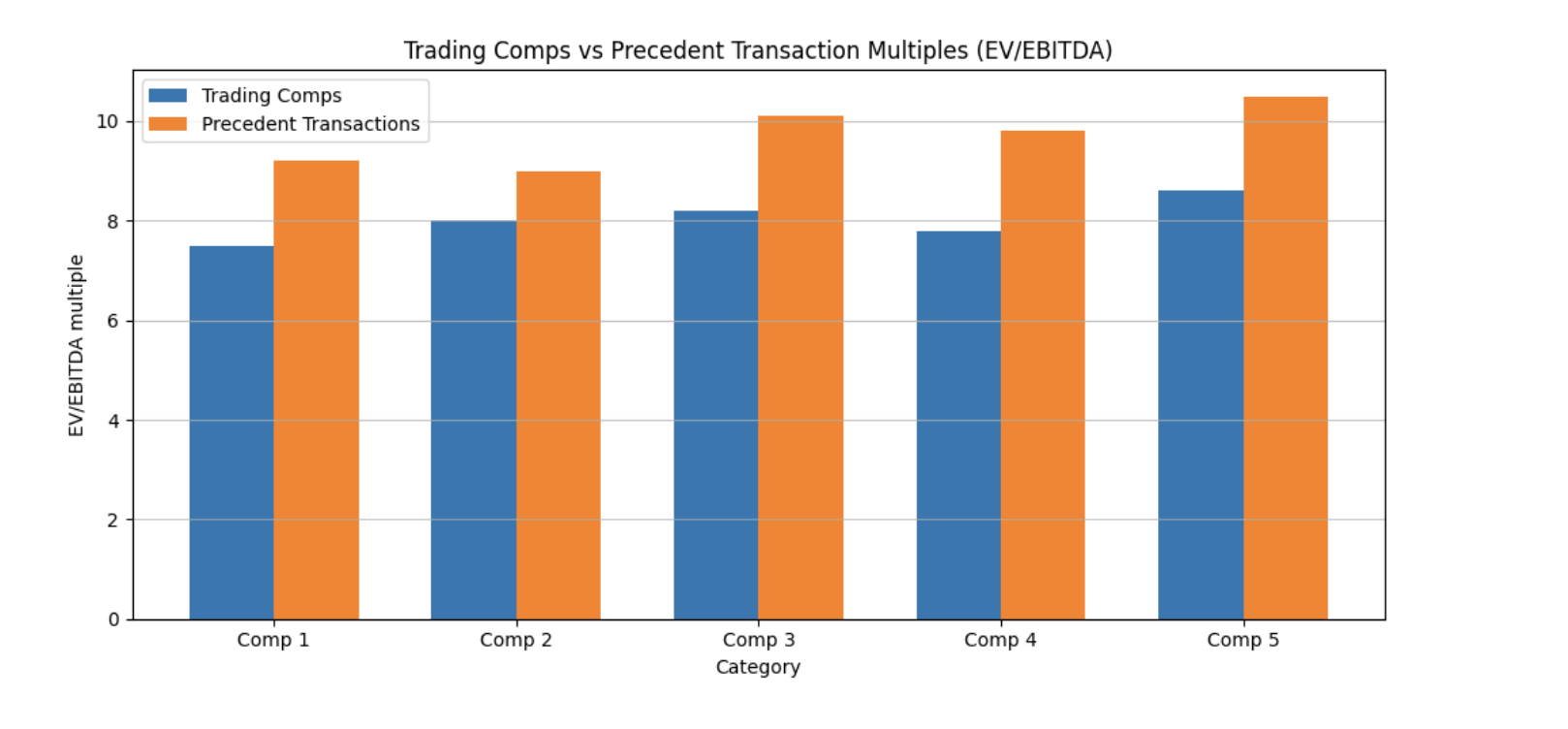
Transaction multiples typically include a control premium, as buyers obtain control over strategy and cash flows. They also embed expected synergies and strategic considerations, as well as prevailing credit-market conditions at the time of the deal.

From a technical standpoint, transaction enterprise value is reconstructed at announcement using the offer price, fully diluted shares, and the target’s net debt and minority interests. Careful alignment between balance-sheet data and LTM operating metrics is essential.

Trading vs precedent multiples
Figure 2 – Comparison between trading comparables and precedent transaction multiples (EV/EBITDA). The illustration is based on a simulated historical sample consistent with PitchBook and Capital IQ deal data. Precedent transactions typically trade at higher multiples due to control premia, synergies and financing conditions.

Why perfect peers almost never exist

Teaching in business schools often presents comparables as firms with identical sector, geography, size and growth. In real M&A practice, this situation is exceptional.

Business models are frequently hybrid. A single firm may combine SaaS subscriptions, recurring managed services and project-based consulting, each with different margin structures and risk profiles.

Accounting reporting rules, such as International Financial Reporting Standards (IFRS) or US GAAP, further reduce comparability. Differences in revenue recognition (IFRS 15), lease accounting (IFRS 16) or capitalization of development costs can materially affect reported EBITDA.

Finally, many relevant competitors are private or embedded within larger groups, making transparent comparison impossible.

Building a defensible comps set in hybrid sectors

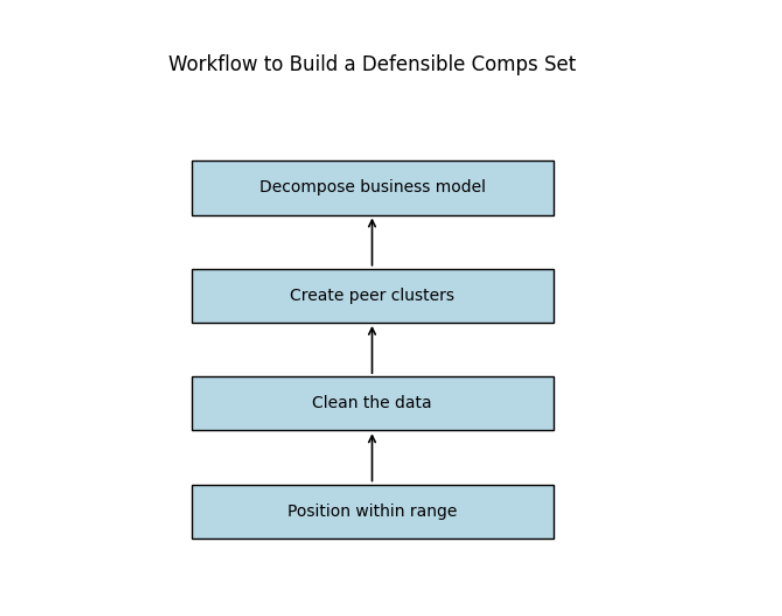
When similarity is weak, the analysis should begin with a decomposition of the target’s business model. Revenue streams are separated into functional blocks (platform, services, consulting), each benchmarked against the most relevant public proxies.

Peer groups are therefore modular rather than homogeneous. Geographic constraints are relaxed progressively, prioritising business-model similarity over local proximity.

Comps workflow
Figure 3 – Bottom-up workflow for constructing a defensible comps set in niche sectors. The figure illustrates the analytical sequence used by practitioners: business-model decomposition, peer clustering, financial cleaning and positioning within a valuation range.

When comparables fail: the role of DCF

When no meaningful peers exist, discounted cash-flow (DCF) analysis becomes the primary valuation tool.

A DCF estimates firm value by projecting free cash flows and discounting them at the weighted average cost of capital (WACC), which reflects the opportunity cost for both debt and equity investors.

Key valuation drivers include unit economics, operating leverage and realistic assumptions on growth and margins. Sensitivity analysis is essential to reflect uncertainty.

Corporate buyers versus private equity sponsors

Corporate acquirers focus on strategic fit and synergies, while private equity sponsors are constrained by required internal rates of return (IRR) and money-on-money multiples (MOIC).

Despite different objectives, both rely on the same principle: when comparables are imperfect, the narrative behind the multiples matters more than the multiples themselves.

How to communicate limitations effectively

From the analyst’s perspective, the key is transparency. Clearly stating the limitations of the comps set and explaining the analytical choices strengthens credibility rather than weakening conclusions.

Useful resources

Damodaran, A. (NYU), Damodaran Online.

Rosenbaum, J. & Pearl, J. (2013), Investment Banking: Valuation, Leveraged Buyouts, and Mergers & Acquisitions, Wiley.

Koller, T., Goedhart, M. & Wessels, D. (2020), Valuation: Measuring and Managing the Value of Companies, McKinsey & Company, 7th edition.

About the author

This article was written in January 2025 by Ian DI MUZIO (ESSEC Business School, Master in Finance (MiF), 2025–2027).

Understanding WACC: a student-friendly guide

Daniel LEE

In this article, Daniel LEE (ESSEC Business School, Global Bachelor in Business Administration (GBBA) – 2023-2027) explains the Weighted Average Cost of Capital (WACC).

Introduction

The Weighted Average Cost of Capital (WACC) is one of the most important concepts in corporate finance and valuation. I know that for some students, it feels abstract or overly technical. In reality, WACC is simpler than we think.

Whether it is a DCF, investment decision or assessing long-term value creation, understanding WACC is essential to interpret the financial world. In a DCF, WACC is used as the discount rate applied for FCF. Moreover, a higher WACC lowers the PV of future cashflows whereas a lower WACC increases the firm value. That is why WACC is a benchmark for value creation.

What is the cost of capital?

Every company needs funding to operate, which comes from two main sources: debt and equity. Debt is provided by banks or bondholders and equity is provided by shareholders. Both expect to be compensated for the risk they take. Shareholders typically require a higher return because they bear greater risk, as they are paid only after all other obligations have been met. In contrast, debt investors mainly expect regular interest payments and face lower risk because they are paid before shareholders in case of financial difficulty. The cost of capital represents the return required by each group of investors, and the Weighted Average Cost of Capital (WACC) combines these required returns into a single percentage.

The cost of capital is the return required by each investor group and WACC combines these two expectations with a simple %.

Breaking down the WACC formula

WACC is calculated with this formula:

Formula for the WACC

To gather these elements, we use several methods such as:

Cost of Equity: CAPM model

Cost of equity = Risk-free rate + β (Expected market return – Risk-free rate)

Beta measures how sensitive a company’s returns are to movements in the overall market. It captures systematic risk, meaning the risk that cannot be eliminated through diversification. A beta above 1 indicates that the firm is more volatile than the market, while a beta below 1 means it is less sensitive to market changes.

It is important to distinguish between unlevered beta and levered beta. The unlevered beta reflects only the risk of the firm’s underlying business activities, assuming the company has no debt. It represents the pure business risk of the firm and is especially useful when comparing companies within the same industry, as it removes the effect of different financing choices. This is why analysts often unlever betas from comparable firms and then relever them to match a target capital structure.

The levered beta, on the other hand, includes both business risk and financial risk created by the use of debt. When a company takes on more debt, shareholders face greater risk because interest payments must be made regardless of the firm’s performance. This increases the volatility of equity returns, leading to a higher levered beta and a higher cost of equity.

The risk-free rate represents the return investors can earn without taking any risk and is usually approximated by long-term government bond yields. It acts as the baseline return in the CAPM, since investors will only accept risky investments if they offer a return above this rate. Choosing the correct risk-free rate is important: it should match the currency and the time horizon of the cash flows. Changes in the risk-free rate have a direct impact on the cost of equity and, therefore, on firm valuation.

Cost of Debt

The interest payments are tax-deductible. That’s why we include 1-T in the formula. For example: if a company pays 5% interest annually and the corporate tax rate is 30% then the net cost of debt is 5%*(1-0.3) = 3.5%.

Capital Structure Weights

The weights Equity/(Equity+Debt) and Debt/(Equity+Debt) represents the proportion of equity and debt in the company’s balance sheet. We can then assume that a firm with more debt will have a lower WACC because debt is cheaper, but too much debt is risky. That is why the balance is very important for valuation and that usually you use a “target capitalization”. Target capitalization is an assumption of the level of debt and equity that a company is expected to have in the long term, rather than the current one.

Understanding risk through the WACC

WACC is a measure of risk. A higher WACC means the company is riskier and a lower WACC means it’s safer.

WACC is also closely linked to a firm’s capability to create value. If ROIC > WACC then the company creates value, but if ROIC < WACC, the company destroys value. This rule is widely used by CFO and investors to take decisions.

How is WACC used in practice?

  • WACC is the discount rate applied to FCF in the DCF > Lower WACC = Higher valuation; Higher WACC = Lower Valuation
  • As said before, it helps to assess value creation and find NPV
  • Assessing capital structure > helps to find the optimal balance between debt and equity
  • Comparing companies > good preliminary step to look at similar companies in the same company, the WACC will tell you a lot about their risk

Example

To illustrate how the WACC formula is used in practice, let us take the DCF valuation for Alstom that I made recently. In this valuation, WACC is used as the discount rate to convert future free cash flows into present value.

Alstom’s capital structure is defined using a target capitalization, that was chosen on the industry and the comps. Equity represents 75% of total capital and debt 25%. The cost of equity is estimated using the CAPM. Based on the base-case assumptions, Alstom has a levered beta that reflects both its industrial business risk and its use of debt. Combined with a risk-free rate and an equity risk premium, this leads to a cost of equity of 8.3%.

The cost of debt is estimated using Alstom’s borrowing conditions. Alstom pays an average interest rate of 4.12% on its debt. Since interest expenses are tax-deductible, we adjust for taxes. With a corporate tax rate of 25.8%, the after-tax cost of debt is:

4.12%×(1-0.258)=3.05%

We can now compute the WACC:

WACC=75%×8.3%+25%×3.05%=6.98%

This WACC represents the minimum return Alstom must generate on its invested capital to satisfy both shareholders and lenders. In the DCF, this rate is applied to discount future free cash flows. A higher WACC would reduce Alstom’s valuation, while a lower WACC would increase it, highlighting how sensitive valuations are to financing assumptions.

Conclusion

To conclude, WACC may look a bit complicated, but it represents a simple idea: the company must generate enough to reward its investors for the risk they take. Understanding WACC allows people to interpret valuations, understand how capital structure influences risk and compare businesses across industries. Once you master the WACC, it is one of the best tools to dig your intuition about risk and valuation.

Related posts on the SimTrade blog

   ▶ Snehasish CHINARA Academic perspectives on optimal debt structure and bankruptcy costs

   ▶ Snehasish CHINARA Optimal capital structure with corporate and personal taxes: Miller 1977

   ▶ Snehasish CHINARA Optimal capital structure with no taxes: Modigliani and Miller 1958

Useful resources

Damodaran, A. (2001) Corporate Finance: Theory and Practice. 2nd edn. New York: John Wiley & Sons.

Modigliani, F., M.H. Miller (1958) The Cost of Capital, Corporation Finance and the Theory of Investment, American Economic Review, 48(3), 261-297.

Modigliani, F., M.H. Miller (1963) Corporate Income Taxes and the Cost of Capital: A Correction, American Economic Review, 53(3), 433-443.

Vernimmen, P., Quiry, P. and Le Fur, Y. (2022) Corporate Finance: Theory and Practice, 6th Edition. Hoboken, NJ: Wiley.

About the author

The article was written in January 2026 by Daniel LEE (ESSEC Business School, Global Bachelor in Business Administration (GBBA) – 2023-2027).

   ▶ Read all articles by Daniel LEE.