
Fixed-income arbitrage strategy

In this article, Youssef LOURAOUI (Bayes Business School, MSc. Energy, Trade & Finance, 2021-2022) presents the fixed-income arbitrage strategy which is a well-known strategy used by hedge funds. The objective of the fixed-income arbitrage strategy is to benefit from trends or disequilibrium in the prices of fixed-income securities using systematic and discretionary trading strategies.
This article is structured as follow: we introduce the fixed-income arbitrage strategy principle. Then, we present a practical case study to grasp the overall methodology of this strategy. We also present a performance analysis of this strategy and compare it a benchmark representing all hedge fund strategies (Credit Suisse Hedge Fund index) and a benchmark for the global equity market (MSCI All World Index).
Introduction
According to Credit Suisse (a financial institution publishing hedge fund indexes), a fixed-income arbitrage strategy can be defined as follows: “Fixed-income arbitrage funds attempt to generate profits by exploiting inefficiencies and price anomalies between related fixed-income securities. Funds limit volatility by hedging out exposure to the market and interest rate risk. Strategies include leveraging long and short positions in similar fixed-income securities that are related either mathematically or economically. The sector includes credit yield curve relative value trading involving interest rate swaps, government securities and futures, volatility trading involving options, and mortgage-backed securities arbitrage (the mortgage-backed market is primarily US-based and over-the-counter)”.
Types of arbitrage
Fixed-income arbitrage makes money based on two main underlying concepts:
Pure arbitrage
Identical instruments should have identical price (this is the law of one price). This could be the case, for instance, of two futures contracts traded on two different exchanges. This mispricing could be used by going long the undervalued contract and short the overvalued contract. This strategy uses to work in the days before the rise of electronic trading. Now, pure arbitrage is much less obvious as information is accessible instantly and algorithmic trading wipe out this kind of market anomalies.
Relative value arbitrage
Similar instruments should have a similar price. The fundamental rationale of this type of arbitrage is the notion of reversion to the long-term mean (or normal relative valuations).
Factors that influence fixed-income arbitrage strategies
We list below the sources of market inefficiencies that fixed-income arbitrage funds can exploit.
Market segmentation
Segmentation is of concern for fixed-income arbitrageurs. In financial institutions, the fixed-income desk is split into different traders looking at specific parts of the yield curve. In this instance, some will focus on very short, dated bonds, others while concentrate in the middle part of the yield curve (2-5y) while other while be looking at the long-end of the yield curve (10-30y).
Regulation
Regulation has an implication in the kind of fixed-income securities a fund can hold in their books. Some legislations regulate actively to have specific exposure to high yield securities (junk bonds) since their probability of default is much more important. The diminished popularity linked to the tight regulation can make the valuation of those bonds more attractive than owning investment grade bonds.
Liquidity
Liquidity is also an important concern for this type of strategy. The more liquid the market, the easier it is to trade and execute the strategy (vice versa).
Volatility
Large market movements in the market can have implications to the profitability of this kind of strategy.
Instrument complexity
Instrument complexity can also be a reason to have fixed-income securities. The events of 2008 are a clear example of how banks and regulators didn’t manage to price correctly the complex instruments sold in the market which were highly risky.
Application of a fixed-income arbitrage
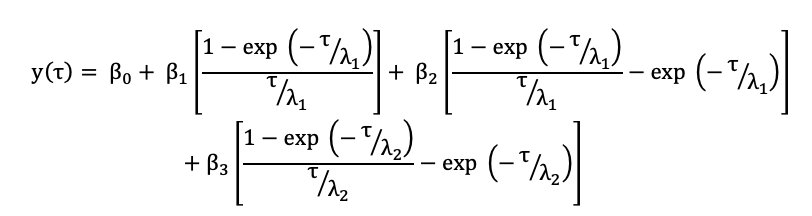
Fixed-income arbitrage strategy makes money by focusing on the liquidity and volatility factors generating risk premia. The strategy can potentially generate returns in both rising and falling markets. However, understanding the yield curve structure of interest rates and detecting the relative valuation differential between fixed-income securities is the key concern since this is what makes this strategy profitable (or not!).
We present below a case study related tot eh behavior of the yield curves in the European fixed-income markets inn the mid 1990’s
The European yield curve differential during in the mid 1990’s
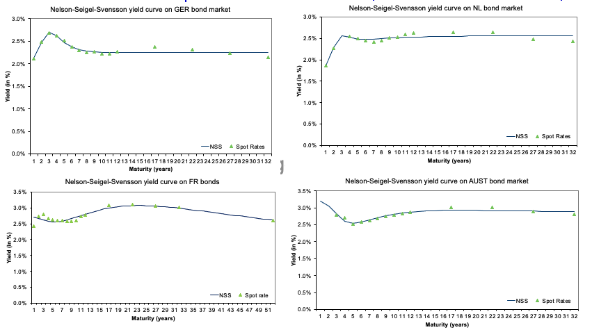
The case showed in this example is the relative-value trade between Germany and Italian yields during the period before the adoption of the Euro as a common currency (at the end of the 1990s). The yield curve should reflect the future path of interest rates. The Maastricht treaty (signed on 7th February 1992) obliged most EU member states to adopt the Euro if certain monetary and budgetary conditions were met. This would imply that the future path of interest rates for Germany and Italy should converge towards the same values. However, the differential in terms of interest rates at that point was nearly 350 bps from 5-year maturity onwards (3.5% spread) as shown in Figure 1.
Figure 1. German and Italian yield curve in January 1995.
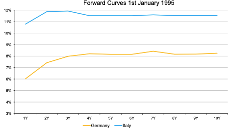
Source: Motson (2022) (Data: Bloomberg).
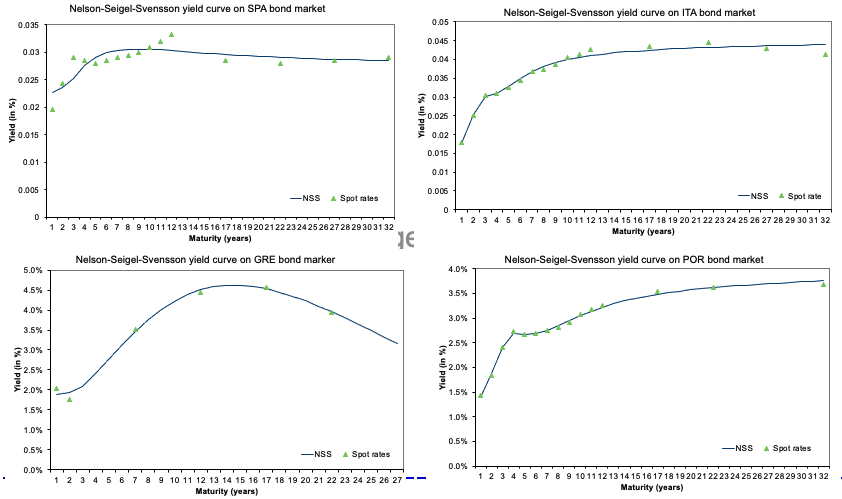
A fixed-income arbitrageur could have profited by entering in an interest rate swap where the investor receives 5y-5y forward Italian rates and pays 5y-5y German rates. If the Euro is introduced, then the spread between the two yield curves for the 5-10y part should converge to zero. As captured in Figure 2, the rates converged towards the same value in 1998, where the spread between the two rates converged to zero.
Figure 2. Payoff of the fixed-income arbitrage strategy.
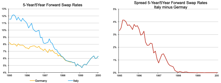
Source: Motson (2022) (Data: Bloomberg).
Performance of the fixed-income arbitrage strategy
Overall, the performance of the fixed-income arbitrage between 1994-2020 were smaller on scale, with occasional large drawdowns (Asian crisis 1998, Great Financial Crisis of 2008, Covid-19 pandemic 2020). This strategy is skewed towards small positive returns but with important tail-risk (heavy losses) according to Credit Suisse (2022). To capture the performance of the fixed-income arbitrage strategy, we use the Credit Suisse hedge fund strategy index. To establish a comparison between the performance of the global equity market and the fixed-income arbitrage strategy, we examine the rebased performance of the Credit Suisse index with respect to the MSCI All-World Index.
Over a period from 2002 to 2022, the fixed-income arbitrage strategy index managed to generate an annualized return of 3.81% with an annualized volatility of 5.84%, leading to a Sharpe ratio of 0.129. Over the same period, the Credit Suisse Hedge Fund index Index managed to generate an annualized return of 5.04% with an annualized volatility of 5.64%, leading to a Sharpe ratio of 0.197. The results are in line with the idea of global diversification and decorrelation of returns derived from the global macro strategy from global equity returns. Overall, the Credit Suisse fixed-income arbitrage strategy index performed better than the MSCI All World Index, leading to a higher Sharpe ratio (0.129 vs 0.08).
Figure 3 gives the performance of the fixed-income arbitrage funds (Credit Suisse Fixed-income Arbitrage Index) compared to the hedge funds (Credit Suisse Hedge Fund index) and the world equity funds (MSCI All-World Index) for the period from July 2002 to April 2021.
Figure 3. Performance of the fixed-income arbitrage strategy.
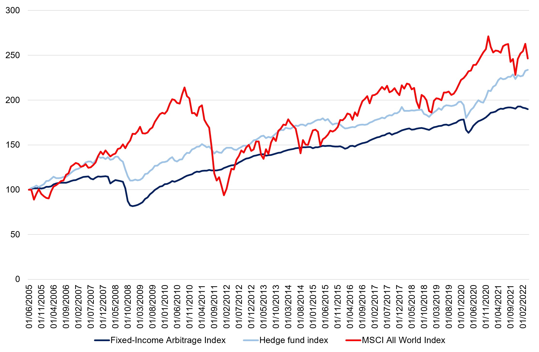
Source: computation by the author (Data: Bloomberg).
You can find below the Excel spreadsheet that complements the explanations about the fixed-income arbitrage strategy.

Why should I be interested in this post?
The fixed-income arbitrage strategy aims to profit from market dislocations in the fixed-income market. This can be implemented, for instance, by investing in inexpensive fixed-income securities that the fund manager predicts that it will increase in value, while simultaneously shorting overvalued fixed-income securities to mitigate losses. Understanding the profits and risks associated with such a strategy may aid investors in adopting this hedge fund strategy into their portfolio allocation.
Related posts on the SimTrade blog
Hedge funds
▶ Youssef LOURAOUI Introduction to Hedge Funds
▶ Youssef LOURAOUI Global macro strategy
▶ Youssef LOURAOUI Long/short equity strategy
Financial techniques
▶ Youssef LOURAOUI Yield curve structure and interest rate calibration
▶ Akshit GUPTA Interest rate swaps
▶ Youssef LOURAOUI Portfolio
Useful resources
Academic research
Pedersen, L. H., 2015. Efficiently Inefficient: How Smart Money Invests and Market Prices Are Determined. Princeton University Press.
Motson, N. 2022. Hedge fund elective. Bayes (formerly Cass) Business School.
Business Analysis
Credit Suisse Hedge fund strategy
Credit Suisse Hedge fund performance
Credit Suisse Fixed-income arbitrage strategy
Credit Suisse Fixed-income arbitrage performance benchmark
About the author
The article was written in January 2023 by Youssef LOURAOUI (Bayes Business School, MSc. Energy, Trade & Finance, 2021-2022).

 Source: www.advratings.com