Portfolio Optimization Archives

Implementing Black-Litterman asset allocation model

March 21, 2022 by Youssef LOURAOUI

In this article, Youssef Louraoui (Bayes Business School, MSc. Energy, Trade & Finance, 2021-2022) presents an implementation of the Black-Litterman model, used to determine the expected return of a portfolio by integrating investor’s views regarding the performance of the underlying assets selected in the investment portfolio.

This article follows the following structure: first, we introduce the Black-Litterman model. We then present the mathematical foundations of this model. We conclude with an explanation of the methodology to build the spreadsheet with the results obtained. You will find in this post an Excel spreadsheet which implement the model.

Introduction

The Black-Litterman asset allocation model, established for the first time in the early 1990’s by Fischer Black and Robert Litterman, is a sophisticated strategy for dealing with unintuitive, highly concentrated, and input-sensitive portfolios. The most likely reason that more portfolio managers do not use the Markowitz model, which maximises return for a given degree of risk, is input sensitivity, a well-documented issue with mean-variance optimization.

The Black-Litterman Model employs a Bayesian technique to integrate an investor’s subjective views of expected returns on one or more assets with the market equilibrium vector (prior distribution) of expected returns to obtain a new, mixed estimate of expected returns. The new vector of returns (the posterior distribution) is a weighted complex average of the investor’s views and market equilibrium.

Mathematical foundation

The idea of the Black Litterman estimates is not to find the optimum portfolio weights as in the Markowitz optimization framework, but instead to find the expected return that would be used as an input to compute the optimum portfolio weights. This approach is referred as reversion portfolio optimization technique. The idea behind is that optimum weights are already observed in the market and captured in the market portfolio. We can approach the reasoning by maximizing the following utility function adjusted to the risk:

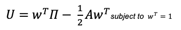
img_SimTrade_mathematical_foundation_Black_Litterman_6

w^T = transposed of portfolio weights
Π = Implied equilibrium excess return vector
A = price of risk or risk aversion factor
Σ = variance-covariance matrix

We take the partial derivative of U in terms of weights (w) and we derive the following expression:

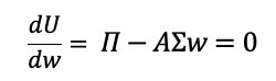
img_SimTrade_mathematical_foundation_Black_Litterman_5

By setting the partial derivative equal to zero, we can maximize the utility function in term of weights. The proposed approach in the Black Litterman approach is that instead of seeking the optimal weights, which are incorporated in the market portfolio and thus computable via the market capitalization of the equities in the portfolio, we’ll isolate the Π (implied equilibrium excess return) to obtain the optimal expected returns for the portfolio:

We can deconstruct the Black-Litterman model as

img_SimTrade_mathematical_foundation_Black_Litterman_3

τ= scalar
P = Linking matrix
∑ = Variance-covariance matrix
Π= implied equilibrium excess return
A = Price of risk
w = weight vector
Ω = uncertainty of views

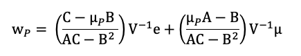
The first term of the formula is introduced in order to respect the constraint that the portfolio weights should be equal to one:

The second term of the formula is to compute a weighted average of the implied equilibrium excess return adjusted to the uncertainty of the returns by the view vector weighted with the uncertainty of views:

The final output E(R) is a vector of return n x 1 that represent the equilibrium returns of the market adjusted to investors views.

Implementation of the Black-Litterman asset allocation model in practice

To model a Black-Litterman portfolio allocation, we obtained a large time series to obtain useful results by downloading the equivalent of 23 years of market data from a data provider (in this example, Bloomberg). We generate the variance-covariance matrix after obtaining all necessary statistical data, which includes the expected return and volatility indicated by the standard deviation of the returns for each stock during the provided period.

The data is derived from the Bloomberg terminal. The first step is to calculate the logarithmic returns and excess returns on the selected assets (returns minus the risk-free rate). After calculating the logarithmic returns on each asset, we can estimate the capital asset pricing model’s returns (CAPM) expected returns. This information will be used to calculate the Black-Litterman expected returns on a comparative basis.

1. The first input for the model is the price of risk A, which represents the risk aversion of investor and is obtained by subtracting the expected return of the market the risk-free rate and divided by the variance of the market:

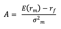
img_SimTrade_Black_Litterman_formulas_for_spreadsheet_1

E(r_m)= expected market returns
r_f = risk-free rate
σ²_m = variance of market

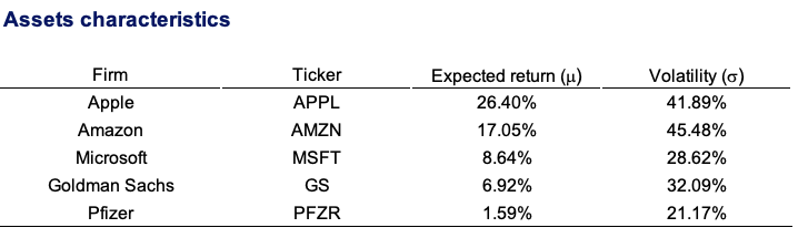
2. We extract the respective market capitalization of each security to obtain their market weights in the portfolio. Given that our investable universe is made of five stocks, we can retrieve their respective market capitalization and compute the weights of each stock in relation to the sum of total market-capitalization in the portfolio.

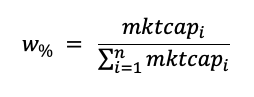
img_SimTrade_Black_Litterman_formulas_for_spreadsheet_2

Table 1 depicts the optimal weights obtained from their respective market capitalisation, coupled with the respective expected return and volatility.

Table 1. Asset characteristics of Apple, Amazon, Microsoft, Goldman Sachs, and Pfizer.

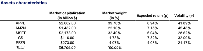
img_SimTrade_Black_Litterman_spreadsheet_2

Source: computation by the author.

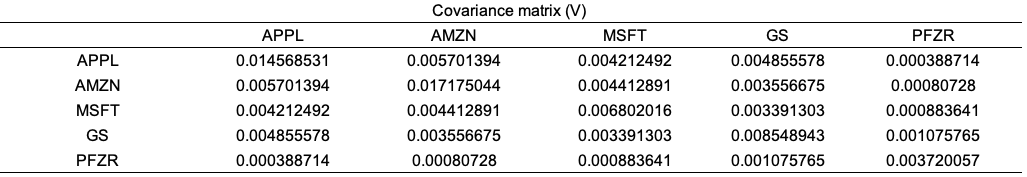
3. We compute the variance-covariance matrix of logarithmic returns using the data analysis tool pack available in Excel (Table 2).

Table 2. Variance-covariance matrix of asset returns

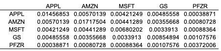
img_SimTrade_Black_Litterman_spreadsheet_5

Source: computation by the author.

4. We compute the implied equilibrium excess return (Π) as the matrix calculation of the price of risk (A) times the matrix multiplication of the weights computed in step 4 times the variance-covariance matrix computed in step 3.

img_SimTrade_Black_Litterman_formulas_for_spreadsheet_3

Π= implied equilibrium excess return
A = Price of risk
w = weight vector

5. The views are incorporated into the model. To achieve this, we provide three views to include into the model. If there are no views, the values will correspond to the market portfolio. The investment manager’s views for the expected return on certain of the portfolio’s assets regularly diverge from the Implied Equilibrium Return Vector (), which serves as the market-neutral starting point for the Black-Litterman model that quantifies the uncertainty associated with each view. The Black-Litterman Model can be used to depict such views in absolute or relative terms. As an illustration, let us suppose that the real and simulated portfolio will have the same views:

View 1: Apple will outperform Microsoft by .05 percent
View 2: Amazon will outperform Microsoft by .1 percent
View 3: Apple will outperform Amazon by .05 percent

To incorporate the vector Q of views, we create a link matrix P where the rows sum to zero. Figure 3 depicts the workings done in the spreadsheet.

Table 3. Views vector and Link Matrix (P)

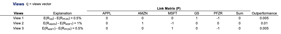
img_SimTrade_Black_Litterman_spreadsheet_1

Source: computation by the author.

6. We compute omega to determine the degree of uncertainty associated with the views. While Black-Litterman paper used a value of tau equal to 0.25, an important number of academics went for calculating the tau equal to one. For the sake of simplifying the model, consider tau to be equal to one. This input is obtained by multiplying the Linking matrix by the variance-covariance matrix and transposing the Linking matrix (P).

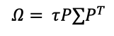
img_SimTrade_Black_Litterman_formulas_for_spreadsheet_4

τ= scalar
P = Linking matrix
∑ = Variance-covariance matrix

7. We integrate all the values computed previously in the Black-Litterman model. Table 4 depicts the results obtained via the Black-Litterman allocation model.

Table 4. Results of the Black-Litterman allocation

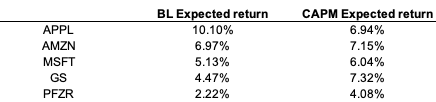
img_SimTrade_Black_Litterman_spreadsheet_4

Source: computation by the author.

We can see that the results converge slightly to those from CAPM. Additionally, we can see that the views are reflected in the Black-Litterman expected returns. As a result, we can determine whether or not each view is satisfied. Indeed, Apple outperforms Amazon and Microsoft, while Amazon outperforms Microsoft.

You can download an Excel file to help you construct a portfolio via the Black-Litterman allocation model.

Why should I be interested in this post?

Modern Portfolio Theory is at the heart of modern finance, shaping the modern investing landscape. MPT has become the cornerstone of current financial theory and practice. MPT’s thesis is that winning the market is difficult and requires diversification and taking higher-than-average risks.

MPT has been around for nearly sixty years and shows no signs of slowing down. His theoretical contributions paved the way for more portfolio theory study. But Markowitz’s portfolio theory is sensitive to and depends on further ‘probabilistic’ expansion. This paper expanded on Markowitz’s previous work by incorporating investor views into the asset allocation process.

Useful resources

Academic research

Black, F. and Litterman, R. 1990. Asset Allocation: Combining Investors Views with Market Equilibrium. Goldman Sachs Fixed Income Research working paper

Black, F. and Litterman, R. 1991. Global Asset Allocation with Equities, Bonds, and Currencies. Goldman Sachs Fixed Income Research working paper

Black, F. and Litterman, R. 1992. Global Portfolio Optimization.Financial Analysts Journal, 28-43.

Idzorek, T.M. 2002. A step-by-step guide to Black-Litterman model. Incorporating user-specified confidence levels. Working Paper, 2-11.

Markowitz, H., 1952. Portfolio Selection. The Journal of Finance, 7(1): 77-91.

About the author

The article was written in Mars 2022 by Youssef LOURAOUI (Bayes Business School, MSc. Energy, Trade & Finance, 2021-2022).

Implementing Markowitz asset allocation model

March 20, 2022 by Youssef LOURAOUI

In this article, Youssef LOURAOUI (Bayes Business School, MSc. Energy, Trade & Finance, 2021-2022) explains how to implement the Markowitz asset allocation model. This model is used to determine optimal asset portfolios based on the risk-return trade-off.

This article follows the following structure: first, we introduce the Markowitz model. We then present the mathematical foundations of this model. We conclude with an explanation of the methodology to build the spreadsheet with the results obtained. You will find in this post an Excel spreadsheet which implements the Markowitz asset allocation model.

Introduction

Markowitz’s work is widely regarded as a pioneer work in financial economics and corporate finance due to its theoretical foundations and applicability in the financial sector. Harry Markowitz received the Nobel Prize in 1990 for his contributions to these disciplines, which he outlined in his 1952 article “Portfolio Selection” published in The Journal of Finance. His major work established the foundation for what is now commonly referred to as “Modern Portfolio Theory” (MPT).

To find the portfolio’s minimal variance, the Markowitz model uses a constrained optimization strategy. The goal of the Markowitz model is to take into account the expected return and volatility of the assets in the investable universe to provide an optimal weight vector that indicates the best allocation for a given level of expected return or the best allocation for a given level of volatility. The expected return, volatility (standard deviation of expected return), and the variance-covariance matrix to reflect the co-movement of each asset in the overall portfolio design are the major inputs for this portfolio allocation model for an n-asset portfolio. We’ll go over how to use this complex method to find the best portfolio weights in the next sections.

Mathematical foundations

The investment universe is composed of N assets characterized by their expected returns μ and variance-covariance matrix V. For a given level of expected return μ_P, the Markowitz model gives the composition of the optimal portfolio. The vector of weights of the optimal portfolio is given by the following formula:

With the following notations:

w_P = vector of asset weights of the portfolio
μ_P = desired level of expected return
e = identity vector
μ = vector of expected returns
V = variance-covariance matrix of returns
V^-1 = inverse of the variance-covariance matrix
t = transpose operation for vectors and matrices

A, B and C are intermediate parameters computed below:

img_SimTrade_implementing_Markowitz_2

The variance of the optimal portfolio is computed as follows

img_SimTrade_implementing_Markowitz_3

To calculate the standard deviation of the optimal portfolio, we take the square root of the variance.

Implementation of the Markowitz asset allocation model in practice

We generated a large time series to obtain useful results by downloading the equivalent of 23 years of market data from a data provider (in this example, Bloomberg). We generate the variance-covariance matrix after obtaining all necessary statistical data, which includes the expected return and volatility indicated by the standard deviation of the returns for each stock during the provided period. Table 1 depicts the expected return and volatility for each stock retained in this analysis.

Table 1. Asset characteristics of Apple, Amazon, Microsoft, Goldman Sachs, and Pfizer.
img_SimTrade_implementing_Markowitz_spreadsheet_1
Source: computation by the author.

We use the data analysis tool pack supplied in Excel to run a variance-covariance matrix for ease of computation (Table 2).

Table 2. Variance-covariance matrix of asset returns.
img_SimTrade_implementing_Markowitz_spreadsheet_4
Source: computation by the author.

We can start the optimization task by setting a desirable expected return after computing the expected return, volatility, and the variance-covariance matrix of expected return. With the data that is fed into the appropriate cells, the model will complete the optimization task. For a 10% desired expected return, we get the following results (Table 3).

Table 3. Asset weights for an optimal portfolio.
img_SimTrade_implementing_Markowitz_spreadsheet_2
Source: computation by the author.

To demonstrate the effect of diversification in the reduction of volatility, we can form a Markowitz efficient frontier by tilting the desired anticipated return with their relative volatility in a graph. The Markowitz efficient frontier is depicted in Figure 1 for various levels of expected return (Figure 1).

Figure 1. Markowitz efficient portfolio frontier.
img_SimTrade_implementing_Markowitz_spreadsheet_3
Source: computation by the author.

You can download the Excel file below to use the Markowitz portfolio allocation model.

Why should I be interested in this post?

Modern Portfolio Theory (MPT) is at the heart of modern finance, shaping the modern investing landscape. MPT has become the cornerstone of current financial theory and practice. MPT has been around for nearly sixty years and shows no signs of slowing down. His theoretical contributions paved the way for more portfolio theories. This post helps you to grasp the theoretical model and its implementation.

Useful resources

Academic research

Petters, A. O., and Dong, X. 2016. An Introduction to Mathematical Finance and Applications. Springer Undergraduate Texts in Mathematics and Technology.

Markowitz, H., 1952. Portfolio Selection. The Journal of Finance, 7(1): 77-91.

About the author

The article was written in Mars 2022 by Youssef LOURAOUI (Bayes Business School, MSc. Energy, Trade & Finance, 2021-2022).

Black-Litterman Model

November 21, 2021 by Youssef LOURAOUI

In this article, Youssef LOURAOUI (Bayes Business School, MSc. Energy, Trade & Finance, 2021-2022) presents the Black-Litterman model, used to determine optimal asset allocation in a portfolio. The Black-Litterman model takes the Markowitz model one step further: it incorporates an investor’s own views in determining asset allocations.

This article is structured as follows: we introduce the Black-Litterman model. We then present the mathematical foundations of the model to understand how the method is derived. We finish with an example to illustrate how we can implement a Black-Litterman asset allocation in practice.

Introduction

The Black-Litterman asset allocation model, developed by Fischer Black and Robert Litterman in the early 1990’s, is a complex method for dealing with unintuitive, highly concentrated, input-sensitive portfolios produced by the Markowitz model. The most likely reason why more portfolio managers do not employ the Markowitz paradigm, in which return is maximized for a given level of risk, is input sensitivity, which is a well-documented problem with mean-variance optimization.

The Black-Litterman model employs a Bayesian technique to integrate an investor’s subjective views on expected returns for one or more assets with the market equilibrium expected returns (prior distribution) of expected returns to get a new, mixed estimate of expected returns. The new vector of expected returns (the posterior distribution) is a complex, weighted average of the investor’s views and the market equilibrium.

The purpose of the Black-Litterman model is to develop stable, mean-variance efficient portfolios based on an investor’s unique insights that overcome the problem of input sensitivity. According to Lee (2000), the Black-Litterman Model “essentially mitigates” the problem of estimating error maximization (Michaud, 1989) by dispersing errors throughout the vector of expected returns.

The vector of expected returns is the most crucial input in mean-variance optimization; yet, Best and Grauer (1991) demonstrate that this input can be very sensitive in the final result. Black and Litterman (1992) and He and Litterman (1999) investigate various potential projections of expected returns in their search for a fair starting point: historical returns, equal “mean” returns for all assets, and risk-adjusted equal mean returns. They demonstrate that these alternate forecasts result in extreme portfolios, which have significant long and short positions concentrated in a small number of assets.

Mathematical foundation of Black-Litterman model

It is important to introduce the Black-Litterman formula and provide a brief description of each of its elements. In the formula below, the integer k is used to represent the number of views and the integer n to express the number of assets in the investment set (NB: the superscript ’ indicates the transpose and -1 indicates the inverse).

Where:

E[R] = New (posterior) vector of combined expected return (n x 1 column vector)
τ = Scalar
Σ = Covariance matrix of returns (n x n matrix)
P = Identifies the assets involved in the views (k x n matrix or 1 x n row vector in the special case of 1 view)
Ω = Diagonal covariance matrix of error terms in expressed views representing the level of confidence in each view (k x k matrix)
П = Vector of implied equilibrium expected returns (n x 1 column vector)
Q = Vector of views (k x 1 column vector)

Traditionally, personal views are used for prior distribution. Then observed data is used to generate a posterior distribution. The Black-Litterman Model assumes implied returns as the prior distribution and personal views alter it. The basic procedure to find the Black-Litterman model is: 1) Find implied returns 2) Formulate investor views 3) Determine what the expected returns are 4) Find the asset allocation for the optimal portfolio.

Black-Litterman asset allocation in practice

An investment manager’s views for the expected return of some of the assets in a portfolio are frequently different from the the Implied Equilibrium Return Vector (Π), which represents the market-neutral starting point for the Black-Litterman model. representing the uncertainty in each view. Such views can be represented in absolute or relative terms using the Black-Litterman Model. Below are three examples of views stated in the Black and Litterman model (1990).

View 1: Merck (MRK) will generate an absolute return of 10% (Confidence of View = 50%).
View 2: Johnson & Johnson (JNJ) will outperform Procter & Gamble (PG) by 3% (Confidence of View = 65%).
View 3: GE (GE) will beat GM (gm), Wal-Mart (WMT), and Exxon (XOM) by 1.5 percent (Confidence of View = 30%).

An absolute view is exemplified by View 1. It instructs the Black-Litterman model to set Merck’s return at 10%.

Views 2 and 3 are relative views. Relative views are more accurate representations of how investment managers feel about certain assets. According to View 2, Johnson & Johnson’s return will be on average 3 percentage points higher than Procter & Gamble’s. To determine if this will have a good or negative impact on Johnson & Johnson in comparison to Procter & Gamble, their respective Implied Equilibrium returns must be evaluated. In general (and in the absence of constraints and other views), the model will tilt the portfolio towards the outperforming asset if the view exceeds the difference between the two Implied Equilibrium returns, as shown in View 2.

View 3 shows that the number of outperforming assets does not have to equal the number of failing assets, and that the labels “outperforming” and “underperforming” are relative terms. Views that include several assets with a variety of Implied Equilibrium returns are less intuitive, generalizing more challenges. In the absence of constraints and other views, the view’s assets are divided into two mini-portfolios: a long and a short portfolio. The relative weighting of each nominally outperforming asset is proportional to that asset’s market capitalization divided by the sum of the market capitalization of the other nominally outperforming assets of that particular view. Similarly, the relative weighting of each nominally underperforming asset is proportional to that asset’s market capitalization divided by the sum of the market capitalizations of the other nominally underperforming assets. The difference between the net long and net short positions is zero. The real outperforming asset(s) from the expressed view may not be the mini-portfolio that receives the good view. In general, the model will overweight the “outperforming” assets if the view is greater than the weighted average Implied Equilibrium return differential.

Why should I be interested in this post?

Modern Portfolio Theory (MPT) is at the heart of modern finance and its core foundations are structuring the modern investing panorama. MPT has established itself as the foundation for modern financial theory and practice. MPT’s premise is that beating the market is difficult, and those that do it by diversifying their portfolios appropriately and accepting higher-than-average investment risks.

MPT has been around for almost sixty years, and its popularity is unlikely to wane anytime soon. Its theoretical contributions have laid the groundwork for more theoretical research in the field of portfolio theory. Markowitz’s portfolio theory, however, is vulnerable to and dependent on continuing ‘probabilistic’ development and expansion. This article shed light on an enhancement of the initial Markowitz work by going a step further: to incorporate the views of the investors in the asset allocation process.

Useful resources

Academic research

Best, M.J., and Grauer, R.R. 1991. On the Sensitivity of Mean-Variance-Efficient Portfolios to Changes in Asset Means: Some Analytical and Computational Results.The Review of Financial Studies, 315-342.

Black, F. and Litterman, R. 1990. Asset Allocation: Combining Investors Views with Market Equilibrium. Goldman Sachs Fixed Income Research working paper

Black, F. and Litterman, R. 1991. Global Asset Allocation with Equities, Bonds, and Currencies. Goldman Sachs Fixed Income Research working paper

Black, F. and Litterman, R. 1992. Global Portfolio Optimization.Financial Analysts Journal, 28-43.

He, G. and Litterman, R. 1999. The Intuition Behind Black-Litterman Model Portfolios. Goldman Sachs Investment Management Research, working paper.

Idzorek, T.M. 2002. A step-by-step guide to Black-Litterman model. Incorporating user-specified confidence levels. Working Paper, 2-11.

Lee, W., 2000, Advanced theory and methodology of tactical asset allocation. Fabozzi and Associates Publications.

Markowitz, H., 1952. Portfolio Selection. The Journal of Finance, 7(1): 77-91.

Michaud, R.O. 1989. The Markowitz Optimization Enigma: Is Optimized Optimal?. Financial Analysts Journal, 31-42.

Mossin, J. 1966. Equilibrium in a Capital Asset Market. Econometrica, 34(4): 768-783.

Sharpe, W.F. 1963. A Simplified Model for Portfolio Analysis. Management Science, 9(2): 277-293.

Sharpe, W.F. 1964. Capital Asset Prices: A Theory of Market Equilibrium under Conditions of Risk. The Journal of Finance, 19(3): 425-442.

About the author

The article was written in November 2021 by Youssef LOURAOUI > (Bayes Business School, MSc. Energy, Trade & Finance, 2021-2022).

Implementing Black-Litterman asset allocation model

Introduction

Mathematical foundation

Implementation of the Black-Litterman asset allocation model in practice

Why should I be interested in this post?

Related posts on the SimTrade blog

Useful resources

Academic research

About the author

Implementing Markowitz asset allocation model

Introduction

Mathematical foundations

Implementation of the Markowitz asset allocation model in practice

Why should I be interested in this post?

Related posts on the SimTrade blog

Useful resources

Academic research

About the author

Black-Litterman Model

Introduction

Mathematical foundation of Black-Litterman model

Black-Litterman asset allocation in practice

Why should I be interested in this post?

Related posts on the SimTrade blog

Useful resources

Academic research

About the author