Interest Rates and M&A: How Market Dynamics Shift When Rates Rise or Fall

 Emanuele BAROLI

In this article, Emanuele BAROLI (MiF 2025–2027, ESSEC Business School) examines how shifts in interest rates shape the M&A market, outlining how deal structures differ when central banks raise versus cut rates.

Context and objective

The purpose is to explain what interest rates are, how they interact with inflation and liquidity, and how these variables shape merger and acquisition (M&A) activity. The intended outcome is an operational lens you can use to read the current monetary cycle and translate it into cost of capital, valuation, financing structure, and execution windows for deals, distinguishing—when useful—between corporate acquirers and private-equity sponsors.

What are interest rates

Interest rates are the intertemporal price of funds. In economic terms they remunerate the deferral of consumption, insure against expected inflation, and compensate for risk. For real decisions the relevant object is the real rate because it governs the trade-off between investing or consuming today versus tomorrow.

Central banks anchor the very short end through the policy rate and the management of system liquidity (reserve remuneration, market operations, balance-sheet policies). Markets then map those signals into the entire yield curve via expectations about future policy settings and required term premia. When liquidity is ample and cheap, risk-free yields and credit spreads tend to compress; when liquidity becomes scarcer or dearer, yields and spreads widen even without a headline change in the policy rate. This transmission, with its usual lags, is the bridge from monetary conditions to firms’ investment choices.

M&A industry — a definition

The M&A industry comprises mergers and acquisitions undertaken by strategic (corporate) acquirers and by financial sponsors. Activity is the joint outcome of several blocks: the cost and elasticity of capital (both debt and equity), expectations about sectoral cash flows, absolute and relative valuations for public and private assets, regulatory and antitrust constraints, and the degree of managerial confidence. Interest rates sit at the center because they enter the denominator of valuation models—through the discount rate—and they shape bankability constraints through the debt service burden. In other words, rates influence both the price a buyer can rationally pay and the feasibility of financing that price.

Use of leverage

Leverage translates a given cash-flow profile into equity returns. In leveraged acquisitions—especially LBOs—the all-in cost of debt is set by a market benchmark (in practice, Term SOFR at three or six months in the U.S., and Euribor in the euro area) plus a spread reflecting credit risk, liquidity, seniority, and the supply–demand balance across channels such as term loans, high-yield bonds, and private credit. That all-in cost determines sustainable leverage, shapes covenant design, and fixes the headroom on metrics like interest coverage and net leverage. It ultimately caps the bid a sponsor can submit while still meeting target returns. Corporate acquirers usually employ more modest leverage, yet remain rate-sensitive because medium-to-long risk-free yields and investment-grade spreads feed both fixed-rate borrowing costs and the WACC used in DCF and accretion tests, and they influence the value of stock consideration in mixed or stock-for-stock deals.

How interest rates impact the M&A industry

The connection from rates to M&A operates through three main channels. The first is valuation: holding cash flows constant, a higher risk-free rate or higher term premia lifts discount rates, lowers present values, and compresses multiples, thereby narrowing the economic room to pay a control premium. The second is bankability: higher benchmarks and wider spreads raise coupons and interest expense, reduce sustainable leverage, and shrink the set of financeable deals—most visibly for sponsors whose equity returns depend on the spread between debt cost and EBITDA growth. The third is market access: heightened rate volatility and tighter liquidity reduce underwriting depth and risk appetite in loans and bonds, delaying signings or closings; the mirror image under easing—lower rates, stable curves, and tighter spreads—reopens windows, enabling new-money term funding and refinancing of maturities. The net effect is a function of level, slope, and volatility of the curve: lower and calmer curves with steady spreads tend to support volumes; high or unstable curves, even with unchanged spreads, enforce selectivity.

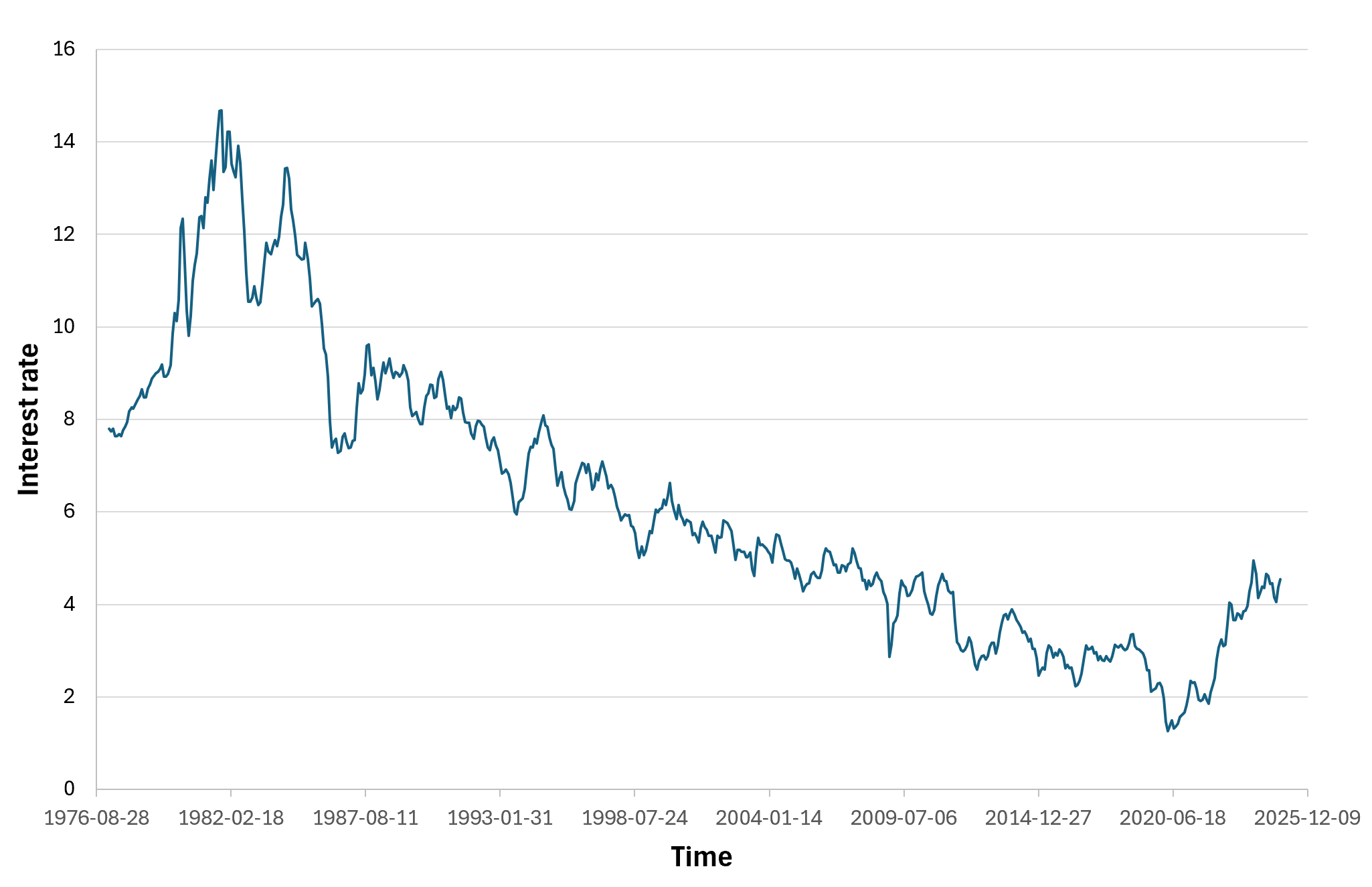
Evidence from 2021–2024 and what the chart shows

M&A deals and interest rates (2021-2024).
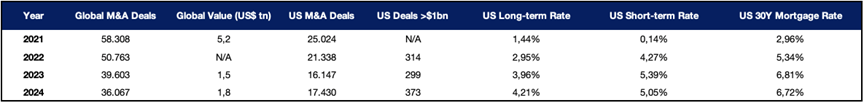
M&A deals and interest rates (2021-2024)
Source: Fed.

The global pattern over 2021–2024 is consistent with this mechanism. In 2021, deal counts reached a cyclical peak in an environment of near-zero short-term rates, abundant liquidity, and elevated equity valuations; frictions on the cost of capital were minimal and access to debt markets was easy, so the economic threshold for completing transactions was lower. Between 2022 and 2024, monetary tightening lifted short-term benchmarks rapidly while spreads and uncertainty rose; global deal counts fell materially and the market became more selective, favoring higher-quality assets, resilient sectors, and transactions with stronger industrial logic. Over this period, global deal counts were 58,308 in 2021, 50,763 in 2022, 39,603 in 2023, and 36,067 in 2024, while U.S. short-term rates moved from roughly 0.14% to above 5%; the chart shows an inverse co-movement between the cost of money and activity. Correlation is not causation—antitrust enforcement, energy shocks, equity multiple swings, and the rise of private credit also mattered—but the macro signal aligns with monetary transmission.

What does academic research say

Academic research broadly confirms the mechanism sketched above: when policy rates rise and financing conditions tighten, both the volume and composition of M&A activity change. Using U.S. data, Adra, Barbopoulos, and Saunders (2020) show that increases in the federal funds rate raise expected financing costs, are followed by more negative acquirer announcement returns, and significantly increase the probability that deals are withdrawn, especially when monetary policy uncertainty is high. Fischer and Horn (2023) and Horn (2021) exploit high-frequency monetary-policy shocks and find that a contractionary shock leads to a persistent fall in aggregate deal numbers and values—on the order of 20–30%—with the effect concentrated among financially constrained bidders; at the same time, the average quality of completed deals improves because weaker acquirers are screened out. Work on leveraged buyouts links this to credit conditions: Axelson et al. (2013) document that cheap and abundant credit is associated with higher leverage and higher buyout prices relative to comparable public firms, while theoretical models such as Nicodano (2023) show how optimal LBO leverage and default risk respond systematically to the level of risk-free rates and credit spreads.

Related posts on the SimTrade blog

   ▶ Bijal GANDHI Interest Rates

   ▶ Nithisha CHALLA Relation between gold price and interest rate

   ▶ Roberto RESTELLI My internship at Valori Asset Management

Useful resources

Academic articles

Adra, S., Barbopoulos, L., & Saunders, A. (2020). The impact of monetary policy on M&A outcomes. Journal of Corporate Finance, 62, 1-61.

Fischer, J. and Horn, C.-W. (2023), Monetary Policy and Mergers and Acquisitions, Working paper Available at SSRN

Horn, C.-W. (2021) Does Monetary Policy Affect Mergers and Acquisitions? Working paper.

Axelson, U., Jenkinson, T., Strömberg, P., & Weisbach, M. S. (2013) Borrow Cheap, Buy High? The Determinants of Leverage and Pricing in Buyouts, The Journal of Finance, 68(6), 2223-2267.

Financial data

Federal Reserve Bank of New York Effective Federal Funds Rate (EFFR): methodology and data

Federal Reserve Bank of St. Louis Effective Federal Funds Rate (FEDFUNDS)

OECD Data Long-term interest rates

About the author

The article was written in November 2025 by Emanuele BAROLI (ESSEC Business School, Master in Finance (MiF), 2025–2027).

   ▶ Read all articles by Emanuele BAROLI.

Treasury Bonds: The Backbone of U.S. Government Financing

Treasury Bonds: The Backbone of U.S. Government Financing

Camille Keller

In this article, Camille KELLER (ESSEC Business School, Bachelor in Business Administration (BBA), 2020-2024) explains the purpose, significance, and global role of U.S. Treasury bonds.

Introduction

Treasury bonds (T-bonds) are long-term debt securities issued by the U.S. Department of the Treasury, fundamental to funding government operations and shaping economic policies. Backed by the “full faith and credit” of the U.S. government, they are regarded globally as benchmarks of stability and reliability.

These bonds play a dual role: domestically, they underpin the financial system and provide risk-free investment options, while globally, they influence capital flows and pricing in international markets. With their long maturities and predictable returns (if hold until maturity), Treasury bonds are a secure haven for investors in times of uncertainty.

This article explores the structure of Treasury bonds, their critical role in monetary policy, and their global significance in maintaining financial stability.

What Are Treasury Bonds and How Do They Work?

Treasury bonds are issued by the U.S. government to finance national projects and repay debt. They have maturities of 10 to 30 years and offer fixed semiannual interest payments, returning the principal amount at maturity.

Figure 1 below gives the evolution of the interest rate of Treasury bonds (30 years of maturity) over the period March 1977 – December 2024 (data from Federal Reserve Bank of St. Louis). You can download the Excel file for the historical data used to build the figure.

Figure 1. Evolution of the US Treasury bonds interest rate.
Evolution of the US Treasury bonds interest rate
Source: Federal Reserve Bank of St. Louis.

These bonds are sold through public auctions, where competitive bidders specify desired yields, and non-competitive bidders accept the auction’s determined rate. This transparent process ensures fair pricing and liquidity, making T-bonds accessible to a wide range of investors.

Treasury bonds are considered among the safest investments globally, given the U.S. government’s ability to generate revenue through taxation and currency issuance. This security makes them a key component of institutional portfolios, particularly for pension funds and central banks looking for low-risk, reliable returns.

In financial markets, T-bonds serve as a benchmark for long-term interest rates. Their yields influence borrowing costs for mortgages, corporate bonds, and loans, directly affecting economic activity. During financial uncertainty, their reputation as safe-haven assets attracts significant demand, reaffirming their stability and importance in global markets.

The Role of Treasury Bonds in Monetary Policy

Treasury bonds are integral to U.S. monetary policy, serving as tools for the Federal Reserve to manage money supply and interest rates. Through open market operations, the Federal Reserve buys or sells Treasury bonds to inject or withdraw liquidity from the financial system. These actions influence borrowing costs and economic activity.

When the Federal Reserve purchases T-bonds, it lowers interest rates, encouraging borrowing and investment. Conversely, selling bonds tightens liquidity and increases rates, curbing inflation and slowing economic growth.

T-bonds are also key indicators of inflation expectations. Fixed coupon payments lose value in inflationary periods, prompting investors to demand higher yields as compensation. Their role as a measure of market sentiment makes them critical in assessing economic conditions.

The yield curve—a graph of yields on Treasury securities of varying maturities—offers further insight. An inverted yield curve, where short-term yields exceed long-term yields, is often a precursor to economic recessions, signaling investor concerns about future growth.

Through these mechanisms, Treasury bonds enable the Federal Reserve to balance economic growth, inflation, and employment, making them indispensable to monetary policy.

Treasury Bonds as a Global Benchmark

Treasury bonds extend their influence far beyond U.S. borders, forming the bedrock of the global financial system. Their stability, liquidity, and dollar-denominated nature make them indispensable to central banks, institutional investors, and sovereign wealth funds worldwide.

Central banks, particularly those in countries like China and Japan, hold large reserves of T-bonds to stabilize exchange rates, manage currency reserves, and hedge against market volatility. Their status as a low-risk investment ensures enduring demand, reinforcing the U.S. dollar’s dominance in global finance.

T-bonds also serve as a benchmark for pricing other financial instruments. Their yields represent the risk-free rate used in valuation models for equities, corporate bonds, and derivatives, shaping investment decisions across markets.

In times of crisis, Treasury bonds attract capital as investors seek security, lowering yields and providing stability to global markets. However, this reliance also introduces vulnerabilities; events like U.S. debt ceiling debates or credit rating downgrades can disrupt global confidence in Treasury securities.

Despite these challenges, the unwavering demand for Treasury bonds highlights their critical role in ensuring liquidity and stability in the international financial system.

Why Should I Be Interested in This Post?

This post is a valuable resource for students and professionals interested in understanding the mechanics of Treasury bonds and their broader implications. It highlights the intersection of government finance, monetary policy, and global markets, offering insights into how these instruments shape economies worldwide.

Related Posts on the SimTrade Blog

   ▶ Georges WAUBERT Introduction to bonds

   ▶ Georges WAUBERT Bond Markets

   ▶ Georges WAUBERT Bond valuation

   ▶ Georges WAUBERT Bond risks

   ▶ Bijal GANDHI Credit Rating

   ▶ Jayati WALIA Credit risk

Useful Resources

U.S. Department of the Treasury

Federal Reserve Economic Data (FRED)

Federal Reserve

About the Author

The article was written in December 2024 by Camille KELLER (ESSEC Business School, Bachelor in Business Administration (BBA), 2020-2024).

Relation between gold price and interest rate

Relation between gold price and interest rate

Nithisha CHALLA

In this article, Nithisha CHALLA (ESSEC Business School, Grande Ecole Program – Master in Management (MiM), 2021-2024) provides an overview of the inverse relationship between gold price and interest rate, and how various factors affect the relation between them.

Introduction

Gold and interest rates often exhibit an inverse relationship, meaning that as interest rates rise, gold prices tend to fall, and vice versa. Unlike stocks or bonds, gold doesn’t generate income (like dividends or interest) and is often used as a hedge against inflation or economic uncertainty. For instance, during the early 1980s, the U.S. Federal Reserve raised interest rates sharply to combat high inflation, leading to a short-term drop in gold prices. In 2022, the Fed’s aggressive rate hikes led to a decrease in gold’s appeal, which resulted in a relatively stable but pressured gold market. However, this relationship is not always straightforward and can be influenced by various factors.

The Inverse Relationship

This refers to the mostly known two factors that cause the inverse relationship between gold price and interest rate, namely opportunity costs and currency exchange rates.

Opportunity Cost

One of the primary reasons for this inverse correlation is the opportunity cost of holding gold. When interest rates rise, traditional investments like bonds and fixed deposits become more attractive due to higher yields. As a result, investors may shift their funds from gold to these higher-yielding assets, reducing demand for gold and consequently its price.

Currency Exchange Rates

Another factor is the impact of interest rates on currency exchange rates. Rising interest rates can strengthen a country’s currency, particularly the US Dollar. A stronger dollar can make gold, which is priced in US dollars, more expensive for international buyers, leading to decreased demand and lower prices.

Or is it a complex relationship?

It is important to note that the relationship between gold and interest rates is not always straightforward. Other factors, such as geopolitical tensions, inflation expectations, and market sentiment, can also influence gold prices. For instance, during periods of economic uncertainty or geopolitical turmoil, investors may seek refuge in gold, even if interest rates are rising.

To navigate this complex relationship, investors should consider the following:

  • Diversification: Gold can be a valuable addition to a diversified portfolio, providing a hedge against inflation and economic uncertainty.
  • Long-Term Perspective: A long-term investment horizon can help mitigate short-term price fluctuations and focus on the underlying value of gold as a store of value.
  • Market Timing: While it’s challenging to accurately predict interest rate movements and their impact on gold prices, investors can consider adjusting their gold holdings based on economic indicators and market sentiment.

The Historical Perspective

Historically, gold has been seen as a hedge against inflation. When inflation rises, the purchasing power of fiat currencies declines, making gold an attractive investment. However, rising interest rates can sometimes counteract this inflationary pressure.

The 1970s

A period of high inflation and economic uncertainty led to a surge in gold prices. However, as central banks tightened monetary policy and interest rates rose, gold prices began to decline.

The 2000s

The global financial crisis of 2008 and subsequent quantitative easing measures by central banks led to a significant increase in gold prices. However, as central banks began to normalize monetary policy in the late 2010s, gold prices declined.

Many people believe that the price of gold is inversely related to interest rates. However, it is only partially true. In fact, gold prices are driven not by nominal rates (which are not adjusted for inflation), but by real rates (which are nominal rates adjusted for inflation). Investors should remember that what really matters for gold are real interest rates, not the federal funds rate or nominal yields.

The chart below represents the relation between real interest rates (the 10-year inflation indexed Treasury rate is a proxy for long-term U.S. real interest rates) and the price of gold for the period 2003-2016. It shows significant negative correlation between real interest rates and the price of gold.

Relation between interest rates and gold price
correlation between interest rates and gold price from 2003-2016
Source: Gold price forecast

The Role of Central Bank Policies

Central banks play a crucial role in influencing interest rates and, consequently, gold prices. When central banks implement expansionary monetary policies, such as quantitative easing, they inject liquidity into the economy, which can lead to higher inflation and increased demand for gold. Conversely, when central banks tighten monetary policy by raising interest rates, they can reduce inflationary pressures and dampen gold demand.

The Impact of Geopolitical Risks

Geopolitical tensions, such as wars, political instability, and trade disputes, can also impact the relationship between gold and interest rates. During periods of heightened geopolitical risk, investors may flock to gold as a safe-haven asset, even if interest rates are rising.

Conclusion

In conclusion, understanding the relationship between gold and interest rates is crucial for investors seeking to optimize their portfolios. By considering the various factors that influence this relationship and adopting a long-term investment perspective, investors can effectively navigate the complexities of the gold market.

Why should I be interested in this post?

Gold has been a key financial asset for centuries, acting as a store of value, a hedge against inflation, and a safe-haven asset during economic crises. Understanding its investment options helps students grasp fundamental market dynamics and investor behavior, especially during periods of economic uncertainty.

Related posts on the SimTrade blog

   ▶ Nithisha CHALLA History of Gold

   ▶ Nithisha CHALLA Gold resources in the world

   ▶ Nithisha CHALLA How to invest in Gold

Useful resources

World Gold Council Gold is moving with rates

Bullion by post Gold price and interest rate relationship

CBS news Here’s how interest rates impact gold prices

APMEX When Do Central Banks Buy Gold & How Do They Affect Prices?

Other

Wikipedia Gold

About the author

The article was written in November 2024 by Nithisha CHALLA (ESSEC Business School, Grande Ecole Program – Master in Management (MiM), 2021-2024).

Fixed-income arbitrage strategy

Fixed-income arbitrage strategy

Youssef LOURAOUI

In this article, Youssef LOURAOUI (Bayes Business School, MSc. Energy, Trade & Finance, 2021-2022) presents the fixed-income arbitrage strategy which is a well-known strategy used by hedge funds. The objective of the fixed-income arbitrage strategy is to benefit from trends or disequilibrium in the prices of fixed-income securities using systematic and discretionary trading strategies.

This article is structured as follow: we introduce the fixed-income arbitrage strategy principle. Then, we present a practical case study to grasp the overall methodology of this strategy. We also present a performance analysis of this strategy and compare it a benchmark representing all hedge fund strategies (Credit Suisse Hedge Fund index) and a benchmark for the global equity market (MSCI All World Index).

Introduction

According to Credit Suisse (a financial institution publishing hedge fund indexes), a fixed-income arbitrage strategy can be defined as follows: “Fixed-income arbitrage funds attempt to generate profits by exploiting inefficiencies and price anomalies between related fixed-income securities. Funds limit volatility by hedging out exposure to the market and interest rate risk. Strategies include leveraging long and short positions in similar fixed-income securities that are related either mathematically or economically. The sector includes credit yield curve relative value trading involving interest rate swaps, government securities and futures, volatility trading involving options, and mortgage-backed securities arbitrage (the mortgage-backed market is primarily US-based and over-the-counter)”.

Types of arbitrage

Fixed-income arbitrage makes money based on two main underlying concepts:

Pure arbitrage

Identical instruments should have identical price (this is the law of one price). This could be the case, for instance, of two futures contracts traded on two different exchanges. This mispricing could be used by going long the undervalued contract and short the overvalued contract. This strategy uses to work in the days before the rise of electronic trading. Now, pure arbitrage is much less obvious as information is accessible instantly and algorithmic trading wipe out this kind of market anomalies.

Relative value arbitrage

Similar instruments should have a similar price. The fundamental rationale of this type of arbitrage is the notion of reversion to the long-term mean (or normal relative valuations).

Factors that influence fixed-income arbitrage strategies

We list below the sources of market inefficiencies that fixed-income arbitrage funds can exploit.

Market segmentation

Segmentation is of concern for fixed-income arbitrageurs. In financial institutions, the fixed-income desk is split into different traders looking at specific parts of the yield curve. In this instance, some will focus on very short, dated bonds, others while concentrate in the middle part of the yield curve (2-5y) while other while be looking at the long-end of the yield curve (10-30y).

Regulation

Regulation has an implication in the kind of fixed-income securities a fund can hold in their books. Some legislations regulate actively to have specific exposure to high yield securities (junk bonds) since their probability of default is much more important. The diminished popularity linked to the tight regulation can make the valuation of those bonds more attractive than owning investment grade bonds.

Liquidity

Liquidity is also an important concern for this type of strategy. The more liquid the market, the easier it is to trade and execute the strategy (vice versa).

Volatility

Large market movements in the market can have implications to the profitability of this kind of strategy.

Instrument complexity

Instrument complexity can also be a reason to have fixed-income securities. The events of 2008 are a clear example of how banks and regulators didn’t manage to price correctly the complex instruments sold in the market which were highly risky.

Application of a fixed-income arbitrage

Fixed-income arbitrage strategy makes money by focusing on the liquidity and volatility factors generating risk premia. The strategy can potentially generate returns in both rising and falling markets. However, understanding the yield curve structure of interest rates and detecting the relative valuation differential between fixed-income securities is the key concern since this is what makes this strategy profitable (or not!).

We present below a case study related tot eh behavior of the yield curves in the European fixed-income markets inn the mid 1990’s

The European yield curve differential during in the mid 1990’s

The case showed in this example is the relative-value trade between Germany and Italian yields during the period before the adoption of the Euro as a common currency (at the end of the 1990s). The yield curve should reflect the future path of interest rates. The Maastricht treaty (signed on 7th February 1992) obliged most EU member states to adopt the Euro if certain monetary and budgetary conditions were met. This would imply that the future path of interest rates for Germany and Italy should converge towards the same values. However, the differential in terms of interest rates at that point was nearly 350 bps from 5-year maturity onwards (3.5% spread) as shown in Figure 1.

Figure 1. German and Italian yield curve in January 1995.
German and Italian yield curve in January 1995
Source: Motson (2022) (Data: Bloomberg).

A fixed-income arbitrageur could have profited by entering in an interest rate swap where the investor receives 5y-5y forward Italian rates and pays 5y-5y German rates. If the Euro is introduced, then the spread between the two yield curves for the 5-10y part should converge to zero. As captured in Figure 2, the rates converged towards the same value in 1998, where the spread between the two rates converged to zero.

Figure 2. Payoff of the fixed-income arbitrage strategy.
Payoff of the fixed-income arbitrage strategy.
Source: Motson (2022) (Data: Bloomberg).

Performance of the fixed-income arbitrage strategy

Overall, the performance of the fixed-income arbitrage between 1994-2020 were smaller on scale, with occasional large drawdowns (Asian crisis 1998, Great Financial Crisis of 2008, Covid-19 pandemic 2020). This strategy is skewed towards small positive returns but with important tail-risk (heavy losses) according to Credit Suisse (2022). To capture the performance of the fixed-income arbitrage strategy, we use the Credit Suisse hedge fund strategy index. To establish a comparison between the performance of the global equity market and the fixed-income arbitrage strategy, we examine the rebased performance of the Credit Suisse index with respect to the MSCI All-World Index.

Over a period from 2002 to 2022, the fixed-income arbitrage strategy index managed to generate an annualized return of 3.81% with an annualized volatility of 5.84%, leading to a Sharpe ratio of 0.129. Over the same period, the Credit Suisse Hedge Fund index Index managed to generate an annualized return of 5.04% with an annualized volatility of 5.64%, leading to a Sharpe ratio of 0.197. The results are in line with the idea of global diversification and decorrelation of returns derived from the global macro strategy from global equity returns. Overall, the Credit Suisse fixed-income arbitrage strategy index performed better than the MSCI All World Index, leading to a higher Sharpe ratio (0.129 vs 0.08).

Figure 3 gives the performance of the fixed-income arbitrage funds (Credit Suisse Fixed-income Arbitrage Index) compared to the hedge funds (Credit Suisse Hedge Fund index) and the world equity funds (MSCI All-World Index) for the period from July 2002 to April 2021.

Figure 3. Performance of the fixed-income arbitrage strategy.
 Global macro performance
Source: computation by the author (Data: Bloomberg).

You can find below the Excel spreadsheet that complements the explanations about the fixed-income arbitrage strategy.

Fixed-income arbitrage

Why should I be interested in this post?

The fixed-income arbitrage strategy aims to profit from market dislocations in the fixed-income market. This can be implemented, for instance, by investing in inexpensive fixed-income securities that the fund manager predicts that it will increase in value, while simultaneously shorting overvalued fixed-income securities to mitigate losses. Understanding the profits and risks associated with such a strategy may aid investors in adopting this hedge fund strategy into their portfolio allocation.

Related posts on the SimTrade blog

Hedge funds

   ▶ Youssef LOURAOUI Introduction to Hedge Funds

   ▶ Youssef LOURAOUI Global macro strategy

   ▶ Youssef LOURAOUI Long/short equity strategy

Financial techniques

   ▶ Youssef LOURAOUI Yield curve structure and interest rate calibration

   ▶ Akshit GUPTA Interest rate swaps

   ▶ Youssef LOURAOUI Portfolio

Useful resources

Academic research

Pedersen, L. H., 2015. Efficiently Inefficient: How Smart Money Invests and Market Prices Are Determined. Princeton University Press.

Motson, N. 2022. Hedge fund elective. Bayes (formerly Cass) Business School.

Business Analysis

Credit Suisse Hedge fund strategy

Credit Suisse Hedge fund performance

Credit Suisse Fixed-income arbitrage strategy

Credit Suisse Fixed-income arbitrage performance benchmark

About the author

The article was written in January 2023 by Youssef LOURAOUI (Bayes Business School, MSc. Energy, Trade & Finance, 2021-2022).

Interest rate term structure and yield curve calibration

Interest rate term structure and yield curve calibration

Youssef_Louraoui

In this article, Youssef LOURAOUI (Bayes Business School,, MSc. Energy, Trade & Finance, 2021-2022) presents the usage of a widely used model for building the yield curve, namely the Nelson-Seigel-Svensson model for interest rate calibration.

This article is structured as follows: we introduce the concept of the yield curve. Next, we present the mathematical foundations of the Nelson-Siegel-Svensson model. Finally, we illustrate the model with practical examples.

Introduction

Fine-tuning the term structure of interest rates is the cornerstone of a well-functioning financial market. For this reason, the testing of various term-structure estimation and forecasting models is an important topic in finance that has received considerable attention for several decades (Lorenčič, 2016).

The yield curve is a graphical representation of the term structure of interest rates (i.e. the relationship between the yield and the corresponding maturity of zero-coupon bonds issued by governments). The term structure of interest rates contains information on the yields of zero-coupon bonds of different maturities at a certain date (Lorenčič, 2016). The construction of the term structure is not a simple task due to the scarcity of zero-coupon bonds in the market, which are the basic elements to estimate the term structure. The majority of bonds traded in the market carry coupons (regular paiement of interests). The yields to maturity of coupon bonds with different maturities or coupons are not immediately comparable. Therefore, a method of measuring the term structure of interest rates is needed: zero-coupon interest rates (i.e. yields on bonds that do not pay coupons) should be estimated from the prices of coupon bonds of different maturities using interpolation methods, such as polynomial splines (e.g. cubic splines) and parsimonious functions (e.g. Nelson-Siegel).

As explained in an interesting paper that I read (Lorenčič, 2016), the prediction of the term structure of interest rates is a basic requirement for managing investment portfolios, valuing financial assets and their derivatives, calculating risk measures, valuing capital goods, managing pension funds, formulating economic policy, making decisions about household finances, and managing fixed income assets . The pricing of fixed income securities such as swaps, bonds and mortgage-backed securities depends on the yield curve. When considered together, the yields of non-defaulting government bonds with different characteristics reveal information about forward rates, which are potentially predictive of real economic activity and are therefore of interest to policy makers, market participants and economists. For instance, forward rates are often used in pricing models and can indicate market expectations of future inflation rates and currency appreciation/depreciation rates. Understanding the relationship between interest rates and the maturity of securities is a prerequisite for developing and testing the financial theory of monetary and financial economics. The accurate adjustment of the term structure of interest rates is the backbone of a well-functioning financial market, which is why the refinement of yield curve modelling and forecasting methods is an important topic in finance that has received considerable attention for several decades (Lorenčič, 2016).

The most commonly used models for estimating the zero-coupon curve are the Nelson-Siegel and cubic spline models. For example, the central banks of Belgium, Finland, France, Germany, Italy, Norway, Spain and Switzerland use the Nelson-Siegel model or a type of its improved extension to fit and forecast yield curves (BIS, 2005). The European Central Bank uses the Sonderlind-Svensson model, an extension of the Nelson-Siegel model, to estimate yield curves in the euro area (Coroneo, Nyholm & Vidova-Koleva, 2011).

Mathematical foundation of the Nelson-Siegel-Svensson model

In this article, we will deal with the Nelson-Siegel extended model, also known as the Nelson-Siegel-Svensson model. These models are relatively efficient in capturing the general shapes of the yield curve, which explains why they are widely used by central banks and market practitioners.

Mathematically, the formula of Nelson-Siegel-Svensson is given by:

img_SimTrade_NSS_equation

where

  • τ = time to maturity of a bond (in years)
  • β0 = parameter to capture for the level factor
  • β1= parameter to capture the slope factor
  • β2 = parameter to capture the curvature factor
  • β3 = parameter to capture the magnitude of the second hump
  • λ1 and λ2 = parameters to capture the rate of exponential decay
  • exp = the mathematical exponential function

The parameters β0, β1, β2, β3, λ1 and λ2 can be calculated with the Excel add-in “Solver” by minimizing the sum of squared residuals between the dirty price (market value, present value) of the bonds and the model price of the bonds. The dirty price is a sum of the clean price, retrieved from Bloomberg, and accrued interest. Financial research propose that the Svensson model should be favored over the Nelson-Siegel model because the yield curve slopes down at the very long end, necessitating the second curvature component of the Svensson model to represent a second hump at longer maturities (Wahlstrøm, Paraschiv, and Schürle, 2022).

Application of the yield curve structure

In financial markets, yield curve structure is of the utmost importance, and it is an essential market indicator for central banks. During my last internship at the Central Bank of Morocco, I worked in the middle office, which is responsible for evaluating risk exposures and profits and losses on the positions taken by the bank on a 27.4 billion euro foreign reserve investment portfolio. Volatility evaluated by the standard deviation, mathematically defined as the deviation of a random variable (asset prices or returns in my example) from its expected value, is one of the primary risk exposure measurements. The standard deviation reveals the degree to which the present return deviates from the expected return. When analyzing the risk of an investment, it is one of the most used indicators employed by investors. Among other important exposures metrics, there is the VaR (Value at Risk) with a 99% confidence level and a 95% confidence level for 1-day and 30-day positions. In other words, the VaR is a metric used to calculate the maximum loss that a portfolio may sustain with a certain degree of confidence and time horizon.

Every day, the Head of the Middle Office arranges a general meeting in which he discusses a global debriefing of the most significant overnight financial news and a debriefing of the middle office desk for “watch out” assets that may present an investment opportunity. Consequently, the team is tasked with adhering to the investment decisions that define the firm, as it neither operates as an investment bank nor as a hedge fund in terms of risk and leverage. As the central bank is tasked with the unique responsibility of safeguarding the national reserve and determining the optimal mix of low-risk assets to invest in, it seeks a good asset strategy (AAA bonds from European countries coupled with American treasury bonds). The investment mechanism is comprised of the segmentation of the entire portfolio into three principal tranches, each with its own features. The first tranche (also known as the security tranche) is determined by calculating the national need for a currency that must be kept safe in order to establish exchange market stability (mostly based on short-term positions in low-risk profile assets) (Liquid and high rated bonds). The second tranche is based on a buy-and-hold strategy and a market approach. The first entails taking a long position on riskier assets than the first tranche until maturity, with no sales during the asset’s lifetime (riskier bonds and gold). The second strategy is based on the purchase and sale of liquid assets with the expectation of better returns.

Participants in the market are accustomed to categorizing the debt of eurozone nations. Germany and the Netherlands, for instance, are regarded as “core” nations, and their debt as safe-haven assets (Figure 1). Due to the stability of their yield spreads, France, Belgium, Austria, Ireland, and Finland are “semi-core” nations (Figure 1). Due to their higher bond yields and more volatile spreads, Spain, Portugal, Italy, and Greece are called “peripheral” (BNP Paribas, 2019) (Figure 2). The 10-year gap represents the difference between a country’s 10-year bond yield and the yield on the German benchmark bond. It is a sign of risk. Therefore, the greater the spread, the greater the risk. Figure 3 represents the yield curve for the Moroccan bond market.

Figure 1. Yield curves for core countries (Germany, Netherlands) and semi-core (France, Austria) of the euro zone.
Yield curves for core countries of the euro zone
Source: computation by the author.

Figure 2. Yield curves for peripheral countries of the euro zone
(Spain, Italy, Greece and Portugal).
Yield curves for semi-core countries of the euro zone
Source: computation by the author.

Figure 3. Yield curve for Morocco.
Yield curve for Morocco
Source: computation by the author.

This example provides a tool comparable to the one utilized by central banks to measure the change in the yield curve. It is an intuitive and simplified model created in an Excel spreadsheet that facilitates comprehension of the investment process. Indeed, it is capable of continuously refreshing the data by importing the most recent quotations (in this case, retrieved from investing.com, a reputable data source).

One observation can be made about the calibration limits of the Nelson-Seigel-Svensson model. In this sense, when the interest rate curve is in negative levels (as in the case of the structure of the Japanese curve), the NSS model does not manage to model negative values, obtaining a result with substantial deviations from spot rates. This can be interpreted as a failure of the NSS calibration approach to model a negative interest rate curve.

In conclusion, the NSS model is considered as one of the most used and preferred models by central banks to obtain the short- and long-term interest rate structure. Nevertheless, this model does not allow to model the structure of the curve for negative interest rates.

Excel file for the calibration model of the yield curve

You can download an Excel file with data to calibrate the yield curve for different countries. This spreadsheet has a special macro to extract the latest data pulled from investing.com website, a reliable source for time-series data.

Download the Excel file to compute yield curve structure

Why should I be interested in this post?

Predicting the term structure of interest rates is essential for managing investment portfolios, valuing financial assets and their derivatives, calculating risk measures, valuing capital goods, managing pension funds, formulating economic policy, deciding on household finances, and managing fixed income assets. The yield curve affects the pricing of fixed income assets such as swaps, bonds, and mortgage-backed securities. Understanding the yield curve and its utility for the markets can aid in comprehending this parameter’s broader implications for the economy as a whole.

Related posts on the SimTrade blog

Hedge funds

   ▶ Youssef LOURAOUI Introduction to Hedge Funds

   ▶ Youssef LOURAOUI Equity market neutral strategy

   ▶ Youssef LOURAOUI Fixed income arbitrage strategy

   ▶ Youssef LOURAOUI Global macro strategy

Financial techniques

   ▶ Bijal GANDHI Interest Rates

   ▶ Akshit GUPTA Interest Rate Swaps

Other

   ▶ Youssef LOURAOUI My experience as a portfolio manager in a central bank

Useful resources

Academic research

Lorenčič, E., 2016. Testing the Performance of Cubic Splines and Nelson-Siegel Model for Estimating the Zero-coupon Yield Curve. NGOE, 62(2), 42-50.

Wahlstrøm, Paraschiv, and Schürle, 2022. A Comparative Analysis of Parsimonious Yield Curve Models with Focus on the Nelson-Siegel, Svensson and Bliss Versions. Springer Link, Computational Economics, 59, 967–1004.

Business Analysis

BNP Paribas (2019) Peripheral Debt Offers Selective Opportunities

About the author

The article was written in January 2023 by Youssef LOURAOUI (Bayes Business School,, MSc. Energy, Trade & Finance, 2021-2022).