In this article, Saral BINDAL (Indian Institute of Technology Kharagpur, Metallurgical and Materials Engineering, 2024-2028 & Research Assistant at ESSEC Business School) explains the concept of historical volatility used in financial markets to represent and measure the changes in asset prices.
Introduction
Volatility in financial markets refers to the degree of variation in an asset’s price or returns over time. Simply put, an asset is considered highly volatile when its price experiences large upward or downward movements, and less volatile when those movements are relatively small.
Volatility plays a central role in finance as an indicator of risk and is widely used in various portfolio and risk management techniques.
In practice, the concept of volatility can be operationalized in different ways: historical volatility and implied volatility. Traders and analysts use historical volatility to understand an asset’s past performance and implied volatility as a forward-looking measure of upcoming uncertainties in the market.
Historical volatility measures the actual variability of an asset’s price over a past period, calculated as the standard deviation of its historical returns. Computed over different periods (say a month), historical volatility allows investors to identify trends in volatility and assess how an asset has reacted to market conditions in the past.
Practical Example: Analysis of the S&P 500 Index
Let us consider the S&P 500 index as an example of the calculation of volatility.
Prices
Figure 1 below illustrates the daily closing price of the S&P 500 index over the period from January 2020 to December 2025.
Figure 1. Daily closing prices of the S&P 500 index (2020-2025).

Source: computation by the author.
Returns
Returns are the percentage gain or loss on the asset’s investment and are generally calculated using one of two methods: arithmetic (simple) or logarithmic (continuously compounded).
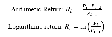
Where Ri represents the rate of return, and Pi denotes the asset’s price at a given point in time.
The preference for logarithmic returns stems from their property of time-additivity, which simplifies multi-period calculations (the monthly log return is equal to the sum of the daily log returns of the month, which is not the case for arithmetic return). Furthermore, logarithmic returns align with the geometric mean thereby mathematically capture the effects of compounding, unlike arithmetic return, which can overstate performance in volatile markets.
Distribution of returns
A statistical distribution describes the likelihood of different outcomes for a random variable. It begins with classifying the data as either discrete or continuous.
Figure 2 below illustrates the distribution of daily returns for S&P 500 index over the period from January 2020 to December 2025.
Figure 2. Historical distribution of daily returns of the S&P 500 index (2020-2025).
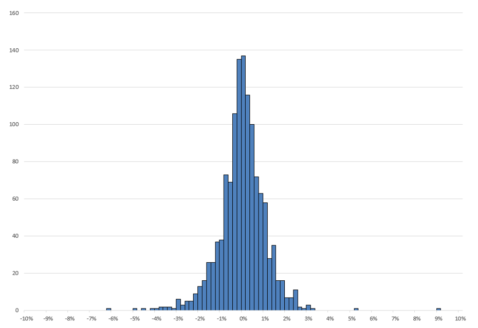
Source: computation by the author.
Standard deviation of the distribution of returns
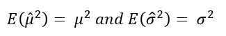
In real life, as we do not know the mean and standard deviation of returns, these parameters have to be estimated with data.
The estimator for the mean μ, denoted by μ̂, and the estimator for the variance σ2, denoted by σ̂2, are given by the following formulas:

With the following notations:
- Ri = rate of return for the ith day
- μ̂ = estimated mean of the data
- σ̂2 = estimated variance of the data
- n = total number of days for the data
These estimators are unbiased and efficient (note the Bessel’s correction for the standard deviation when we divide by (n–1) instead of n).
For the distribution of returns in Figure 2, the mean and standard deviation calculated using the formulas above are 0.049% and 1.068%, respectively (in daily units).
Annualized volatility
As the usual time frame for human is the year, volatility is often annualized. In order to obtain annual (or annualized) volatility, we scale the daily volatility by the square root of the number of days in that period (τ), as shown below.
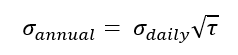
Where is the number of trading days during the calendar year.
In the U.S. equity market, the annual number of trading days typically ranges from 250 to 255 (252 tradings days in 2025). This variation reflects the holiday calendar: when a holiday falls on a weekday, the exchange closes ; when it falls on a weekend, trading is unaffected. In contrast, the cryptocurrency market has as many trading days as there are calendar days in a year, since it operates continuously, 24/7.
For the S&P 500 index over the period from January 2020 to December 2025, the annualized volatility is given by

Annualized mean
The calculated mean for the 5-year S&P 500 logarithmic returns is also the daily average return for the period. The annualized average return is given by the formula below.
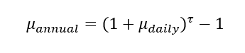
Where τ is the number of trading days during the calendar year.
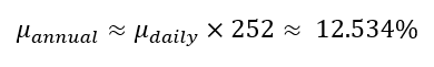
For the S&P 500 index over the period from January 2020 to December 2025, the annualized average return is given by

If the value of daily average return is much less than 1, annual average return can be approximated as
Application: Estimating the Future Price Range of the S&P 500 index
To develop an intuitive understanding of these figures, we can estimate the one-standard-deviation price range for the S&P 500 index over the next year. From the above calculations, we know that the annualized mean return is 12.534% and the annualized standard deviation is 16.953%.
Under the assumption of normally distributed logarithmic returns, we can say approximately with 68% confidence that the value of S&P 500 index is likely to be in the range of:
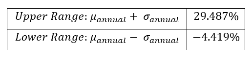
If the current value of the S&P 500 index is $6,830, then converting these return estimates into price levels gives:
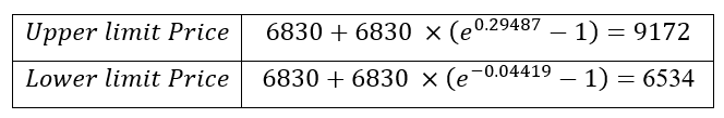
Based on a 68% confidence interval, the S&P 500 index is likely to trade in the range of $6,526 to $8,838 over the next year.
Historical Volatility
Historical volatility represents the variability of an asset’s returns over a chosen lookback period. The annualized historical volatility is estimated using the formula below.
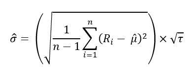
With the following notations:
- σ = Standard deviation
- Ri = Return
- n = total number of trading days in the period (21 for 1 month, 63 for 3 months, etc.)
- τ = Number of trading days in a calendar year
Volatility calculated over different periods must be annualized to a common timeframe to ensure comparability, as the standard convention in finance is to express volatility on an annual basis. Therefore, when working with daily returns, we annualize the volatility by multiplying it by the square root of 252.
For example, for the S&P 500 index, the annualized historical volatilities over the last 1 month, 3 months, and 6 months, computed on December 3, 2025, are 14.80%, 12.41%, and 11.03%, respectively. The results suggest, since the short term (1 month) volatility is higher than medium (3 months) and long term (6 months) volatility, the recent market movements have been turbulent as compared to the past few months, and due to volatility clustering, periods of high volatility often persist, suggesting that this elevated turbulence may continue in the near term.
Unconditional Volatility
Unconditional volatility is a single volatility number using all historical data, which in our example is the entire five years data; It does not account for the fact that recent market behavior is more relevant for predicting tomorrow’s risk than events from past years, implying that volatility changes over time. It is frequently observed that after any sudden boom or crash in the market, as the storm passes away the volatility tends to revert to a constant value and that value is given by the unconditional volatility of the entire period. This tendency is referred to as mean reversion.
For instance, using S&P 500 index data from 2020 to 2025, the unconditional volatility (annualized standard deviation) is calculated to be 16.952%.
Rolling historical volatility
A single volatility number often fails to capture changing market regimes. Therefore, a rolling historical volatility is usually generated to track the evolution of market risk. By calculating the standard deviation over a moving window, we can observe how volatility has expanded or contracted historically. This is illustrated in Figure 3 below for the annualized 3-month historical volatility of the S&P 500 index over the period 2020-2025.
Figure 3. 3-month rolling historical volatility of the S&P500 index (2020-2025).
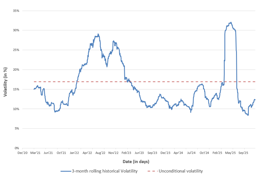
Source: computation by the author.
In Figure 3, the 3-month rolling historical volatility is plotted along with the unconditional volatility computed over the entire period, calculated using overlapping windows to generate a continuous series. This provides a clear historical perspective, showcasing how the asset’s volatility has fluctuated relative to its long-term average.
For example, during the start of Russia–Ukraine war (February 2022 – August 2022), a noticeable jump in volatility occurred as energy and food prices surged amid fears of supply chain disruptions, given that Russia and Ukraine are major exporters of oil, natural gas, wheat, and other commodities.
The rolling window can be either overlapping or non-overlapping, resulting in continuous or discrete graphs, respectively. Overlapping windows shift by one day, creating a smooth and continuous volatility series, whereas non-overlapping windows shift by one time period, producing a discrete series.
You can download the Excel file provided below, which contains the computation of returns, their historical distribution, the unconditional historical volatility, and the 3-month rolling historical volatility of the S&P 500 index used in this article.

You can download the Python code provided below, which contains the computation of returns, first four moments of the distribution, and experiment with the x-month rolling historical volatility function to visualize the evolution of historical volatility over time.

Alternatively, you can download the R code below with the same functionality as in the Python file.

Alterative measures of volatility
We now mention a few other ways volatility can be measured: Parkinson volatility, Implied volatility, ARCH model, and stochastic volatility model.
Parkinson volatility
The Parkinson model (1980) uses the highest and lowest prices during a given period (say a month) for the purpose of measurement of volatility. This model is a high-low volatility measure, based on the difference between the maximum and minimum prices observed during a certain period.
Parkinson volatility is a range-based variance estimator that replaces squared returns with the squared high–low log price range, scaled to remain unbiased. It assumes a driftless (expected growth rate of the stock price equal to zero) geometric Brownian motion, it is five times more efficient than close-to-close returns because it accounts for fluctuation of stock price within a day.
For a sample of n observations (say days), the Parkinson volatility is given by
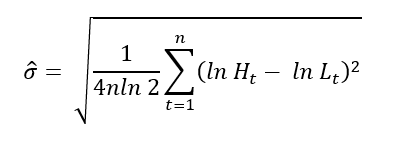
where:
- Ht is the highest price on period t
- Lt is the lowest price on period t
Implied volatility
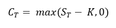
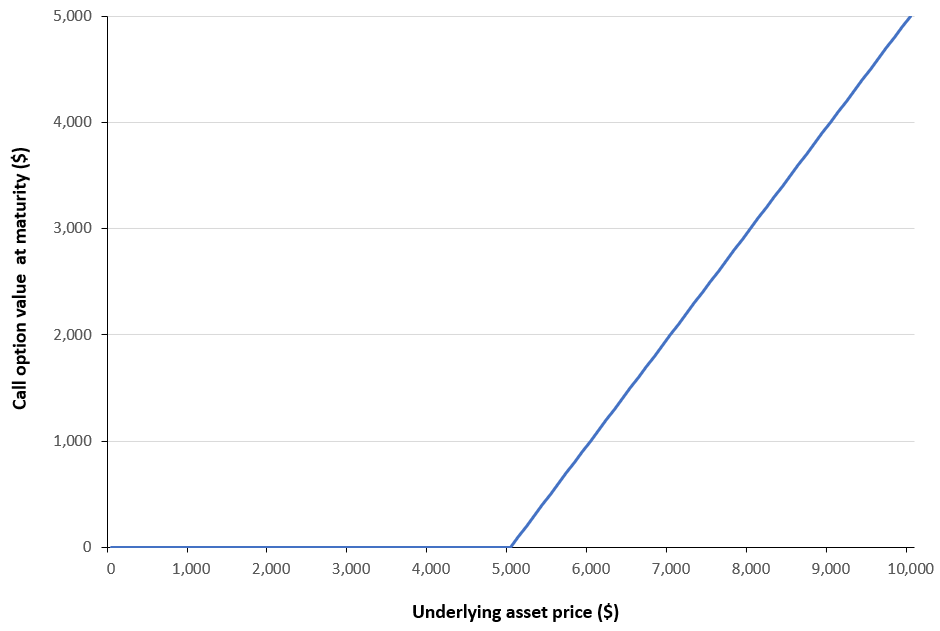
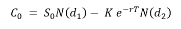
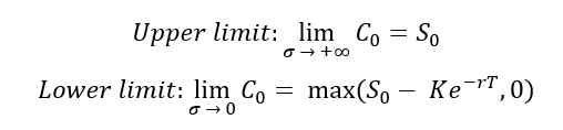
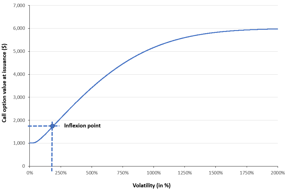
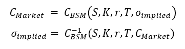
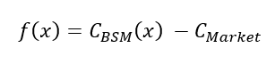
Implied Volatility (IV) is the level of volatility for the underlying asset that, when plugged into an option pricing model such as Black–Scholes–Merton, makes the model’s theoretical option price equal to the option’s observed market price.
It is a forward looking measure because it reflects the market’s expectation of how much the underlying asset’s price is likely to fluctuate over the remaining life of the option, rather than how much it has moved in the past.
The Chicago Board Options Exchange (CBOE), a leading global financial exchange operator provides implied volatility indices like the VIX and Implied Correlation Index, measuring 30-day expected volatility from SPX options. These are used by traders to gauge market fear, speculate via futures/options/ETPs, hedge equity portfolios and manage risk during volatility spikes.
ARCH model
Autoregressive Conditional Heteroscedasticity (ARCH) models address time-varying volatility in time series data. Introduced by Engle in 1982, ARCH models look at the size of past shocks to estimate how volatile the next period is likely to be. If recent movements were big, the model expects higher volatility; if they were small, it expects lower volatility justifying the idea of volatility clustering. Originally applied to inflation data, this model has been widely used in to model financial data.
ARCH model capture volatility clustering, which refers to an observation about how volatility behaves in the short term, a large movement is usually followed by another large movement, thus volatility is predictable in the short term. Historical volatility gives a short-term hint of the near future changes in the market because recent noise often continues.
Generalized Autoregressive Conditional Heteroscedasticity (GARCH) extends ARCH by past predicted volatility, not just past shocks, as refined by Bollerslev in 1986 from Engle’s work. Both of these methods are more accurate methods to forecast volatility than what we had discussed as they account for the time varying nature of volatility.
Stochastic volatility models
In practice, volatility is time-varying: it exhibits clustering, persistence, and mean reversion. To capture these empirical features, stochastic volatility (SV) models treat volatility not as a constant parameter but as a stochastic process jointly evolving with the asset price. Among these models, the Heston (1993) specification is one of the most influential.
The Heston model assumes that the asset price follows a diffusion process analogous to geometric Brownian motion, while the instantaneous variance evolves according to a mean-reverting square-root process. Moreover, the innovations to the price and variance processes are correlated, thereby capturing the leverage effect frequently observed in equity markets.
Applications in finance
This section covers key mathematical concepts and fundamental principles of portfolio management, highlighting the role of volatility in assessing risk.
The normal distribution
The normal distribution is one of the most commonly used probability distribution of a random variable with a unimodal, symmetric and bell-shaped curve. The probability distribution function for a random variable X following a normal distribution with mean μ and variance σ2 is given by

A random variable X is said to follow standard normal distribution if its mean is zero and variance is one.
The figure below represents the confidence intervals, showing the percentage of data falling within one, two, and three standard deviations from the mean.
Figure 4. Probability density function and confidence intervals for a standard normal varaible.
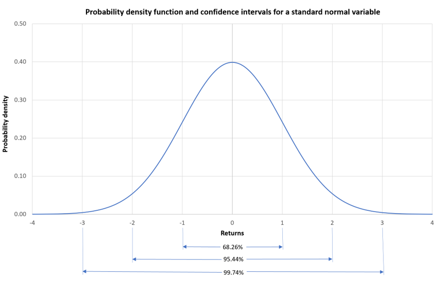
Source: computation by the author
Brownian motion
Robert Brown first observed Brownian motion was as the erratic and random movement of pollen particles suspended in water due to constant collision with water molecules. It was later formulated mathematically by Norbert Wiener and is also known as the Wiener process.
The random walk theory suggests that it’s impossible to predict future stock prices as they move randomly, and when the timestep of this theory becomes infinitesimally small it becomes, Brownian Motion.
In the context of financial stochastic process, when the market is modeled by the standard Brownian motion, the probability distribution function of the future price is a normal distribution, whereas when modeled by Geometric Brownian Motion, the future prices are said to be lognormally distributed. This is also called the Brownian Motion hypothesis on the movement of stock prices.
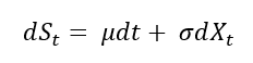
The process of a standard Brownian motion is given by:
The process of a geometric Brownian motion is given by:
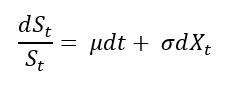
Where, dSt is the change in asset price in continuous time dt, dXt is a random variable from the normal distribution (N (0, 1)) or Wiener process at a time t, σ represents the price volatility, and μ represents the expected growth rate of the asset price, also known as the ‘drift’.
Modern Portfolio Theory (MPT)
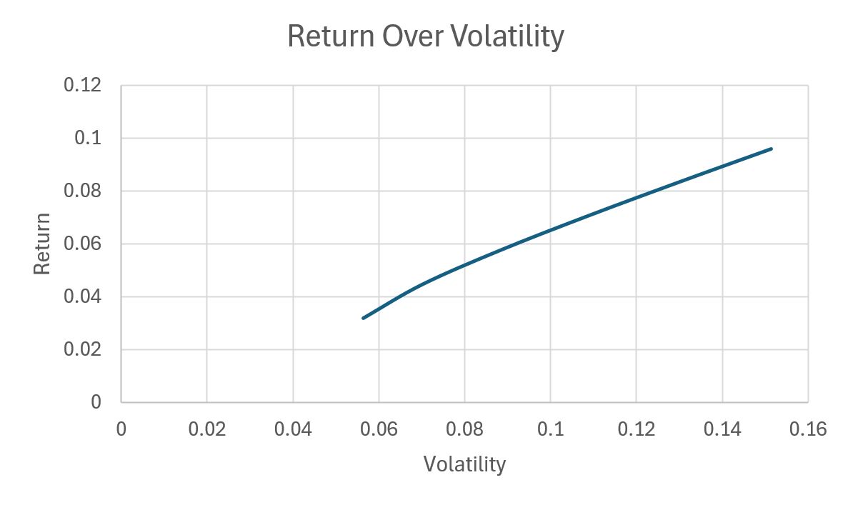
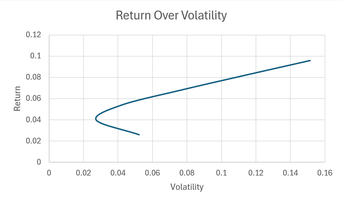
Modern Portfolio Theory (MPT), developed by Nobel Laureate, Harry Markowitz, in the 1950s, is a framework for constructing optimal investment portfolios, derived from the foundational mean-variance model.
The Markowitz mean–variance model suggests that risk can be reduced through diversification. It proposes that risk-averse investors should optimize their portfolios by selecting a combination of assets that balances expected return and risk, thereby achieving the best possible return for the level of risk they are willing to take. The optimal trade-off curve between expected return and risk, commonly known as the efficient frontier, represents the set of portfolios that maximizes expected return for each level of standard deviation (risk).
Capital Asset Pricing Model (CAPM)
The Capital Asset Pricing Model (CAPM) builds on the model of portfolio choice developed by Harry Markowitz (1952), stated above. CAPM states that, assuming full agreement on return distributions and either risk-free borrowing/lending or unrestricted short selling, the value-weighted market portfolio of risky assets is mean-variance efficient, and expected returns are linear in the market beta.
The main result of the CAPM is a simple mathematical formula that links the expected return of an asset to its risk measured by the beta of the asset:
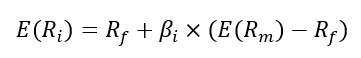
Where:
- E(Ri) = expected return of asset i
- Rf = risk-free rate
- βi = measure of the risk of asset i
- E(Rm) = expected return of the market
- E(Rm) − Rf = market risk premium
CAPM recognizes that an asset’s total risk has two components: systematic risk and specific risk, but only systematic risk is compensated in expected returns.
Returns decomposition fromula.
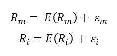
Where the realized (actual) returns of the market (Rm) and the asset (Ri) exceed their expected values only because of consideration of systematic risk (ε).
Decomposition of risk.
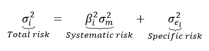
Systematic risk is a macro-level form of risk that affects a large number of assets to one degree or another, and therefore cannot be eliminated. General economic conditions, such as inflation, interest rates, geopolitical risk or exchange rates are all examples of systematic risk factors.
Specific risk (also called idiosyncratic risk or unsystematic risk), on the other hand, is a micro-level form of risk that specifically affects a single asset or narrow group of assets. It involves special risk that is unconnected to the market and reflects the unique nature of the asset. For example, company specific financial or business decisions which resulted in lower earnings and affected the stock prices negatively. However, it did not impact other asset’s performance in the portfolio. Other examples of specific risk might include a firm’s credit rating, negative press reports about a business, or a strike affecting a particular company.
Why should I be interested in this post?
Understanding different measures of volatility, is a pre-requisite to better assess potential losses, optimize portfolio allocation, and make informed decisions to balance risk and expected return. Volatility is fundamental to risk management and constructing investment strategies.
Related posts on the SimTrade blog
Risk and Volatility
▶ Jayati WALIA Brownian Motion in Finance
▶ Youssef LOURAOUI Systematic Risk
▶ Youssef LOURAOUI Specific Risk
▶ Jayati WALIA Implied Volatility
▶ Mathias DUMONT Pricing Weather Risk
▶ Jayati WALIA Black-Scholes-Merton Option Pricing Model
Portfolio Theory and Models
▶ Jayati WALIA Returns
▶ Youssef LOURAOUI Portfolio
▶ Jayati WALIA Capital Asset Pricing Model (CAPM)
▶ Youssef LOURAOUI Optimal Portfolio
Financial Indexes
▶ Nithisha CHALLA Financial Indexes
▶ Nithisha CHALLA Calculation of Financial Indexes
▶ Nithisha CHALLA The S&P 500 Index
Useful Resources
Academic research
Bollerslev, T. (1986). Generalized Autoregressive Conditional Heteroskedasticity, Journal of Econometrics, 31(3), 307–327.
Engle, R. F. (1982). Autoregressive Conditional Heteroscedasticity with Estimates of the Variance of United Kingdom Inflation, Econometrica, 50(4), 987–1007.
Fama, E. F., & French, K. R. (2004). The Capital Asset Pricing Model: Theory and Evidence, Journal of Economic Perspectives, 18(3), 25–46.
Heston, S. L. (1993). A Closed-Form Solution for Options with Stochastic Volatility with Applications to Bond and Currency Options, The Journal of Finance, 48(3), 1–24.
Markowitz, H. M. (1952). Portfolio Selection, The Journal of Finance, 7(1), 77–91.
Parkinson, M. (1980). The extreme value method for estimating the variance of the rate of return. Journal of Business, 53(1), 61–65.
Sharpe, W. F. (1964). Capital Asset Prices: A Theory of Market Equilibrium under Conditions of Risk, The Journal of Finance, 19(3), 425–442.
Tsay, R. S. (2010). Analysis of financial time series, John Wiley & Sons.
Other
NYU Stern Volatility Lab Volatility analysis documentation.
Extreme Events in Finance Risk maps: extreme risk, risk and performance.
About the author
The article was written in December 2025 by Saral BINDAL (Indian Institute of Technology Kharagpur, Metallurgical and Materials Engineering, 2024-2028 & Research Assistant at ESSEC Business School).
▶ Discover all articles written by Saral BINDAL