In this article, Jayati WALIA (ESSEC Business School, Grande Ecole – Master in Management, 2019-2022) presents the variance-covariance method for VaR calculation.
Introduction
VaR is typically defined as the maximum loss which should not be exceeded during a specific time period with a given probability level (or ‘confidence level’). VaR is used extensively to determine the level of risk exposure of an investment, portfolio or firm and calculate the extent of potential losses. Thus, VaR attempts to measure the risk of unexpected changes in prices (or return rates) within a given period.
The two key elements of VaR are a fixed period of time (say one or ten days) over which risk is assessed and a confidence level which is essentially the probability of the occurrence of loss-causing event (say 95% or 99%). There are various methods used to compute the VaR. In this post, we discuss in detail the variance-covariance method for computing value at risk which is a parametric method of VaR calculation.
Assumptions
The variance-covariance method uses the variances and covariances of assets for VaR calculation and is hence a parametric method as it depends on the parameters of the probability distribution of price changes or returns.
The variance-covariance method assumes that asset returns are normally distributed around the mean of the bell-shaped probability distribution. Assets may have tendency to move up and down together or against each other. This method assumes that the standard deviation of asset returns and the correlations between asset returns are constant over time.
VaR for single asset
VaR calculation for a single asset is straightforward. From the distribution of returns calculated from daily price series, the standard deviation (σ) under a certain time horizon is estimated. The daily VaR is simply a function of the standard deviation and the desired confidence level and can be expressed as:
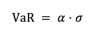
Where the parameter ɑ links the quantile of the normal distribution and the standard deviation: ɑ = 2.33 for p = 99% and ɑ = 1.645 for p = 90%.
In practice, the variance (and then the standard deviation) is estimated from historical data.
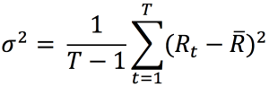
Where Rt is the return on period [t-1, t] and R the average return.
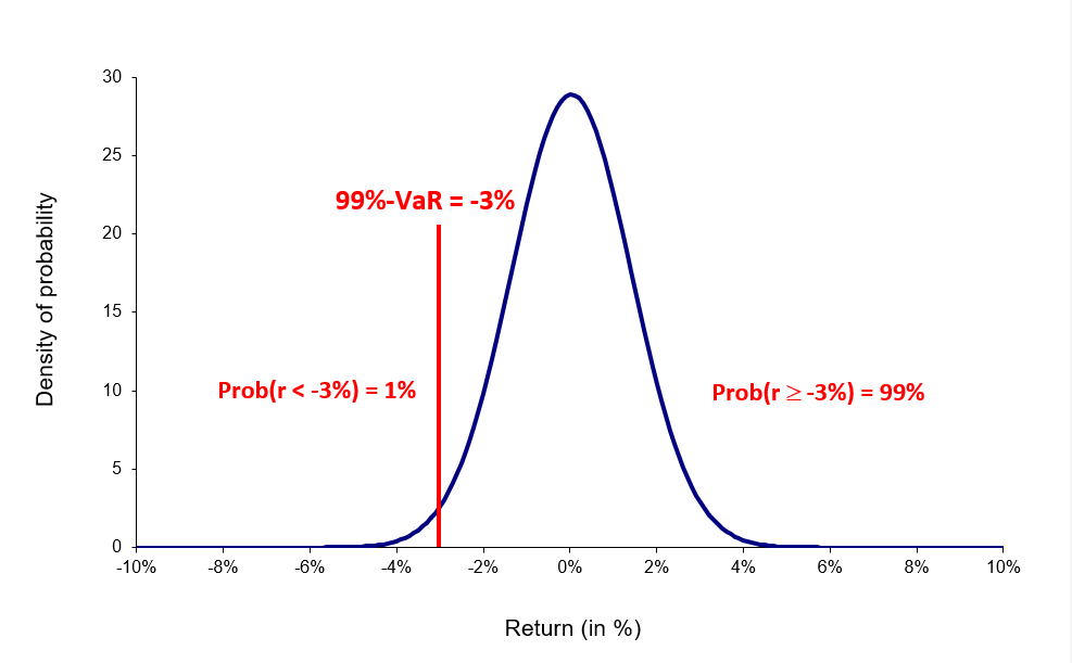
Figure 1. Normal distribution for VaR for the CAC40 index
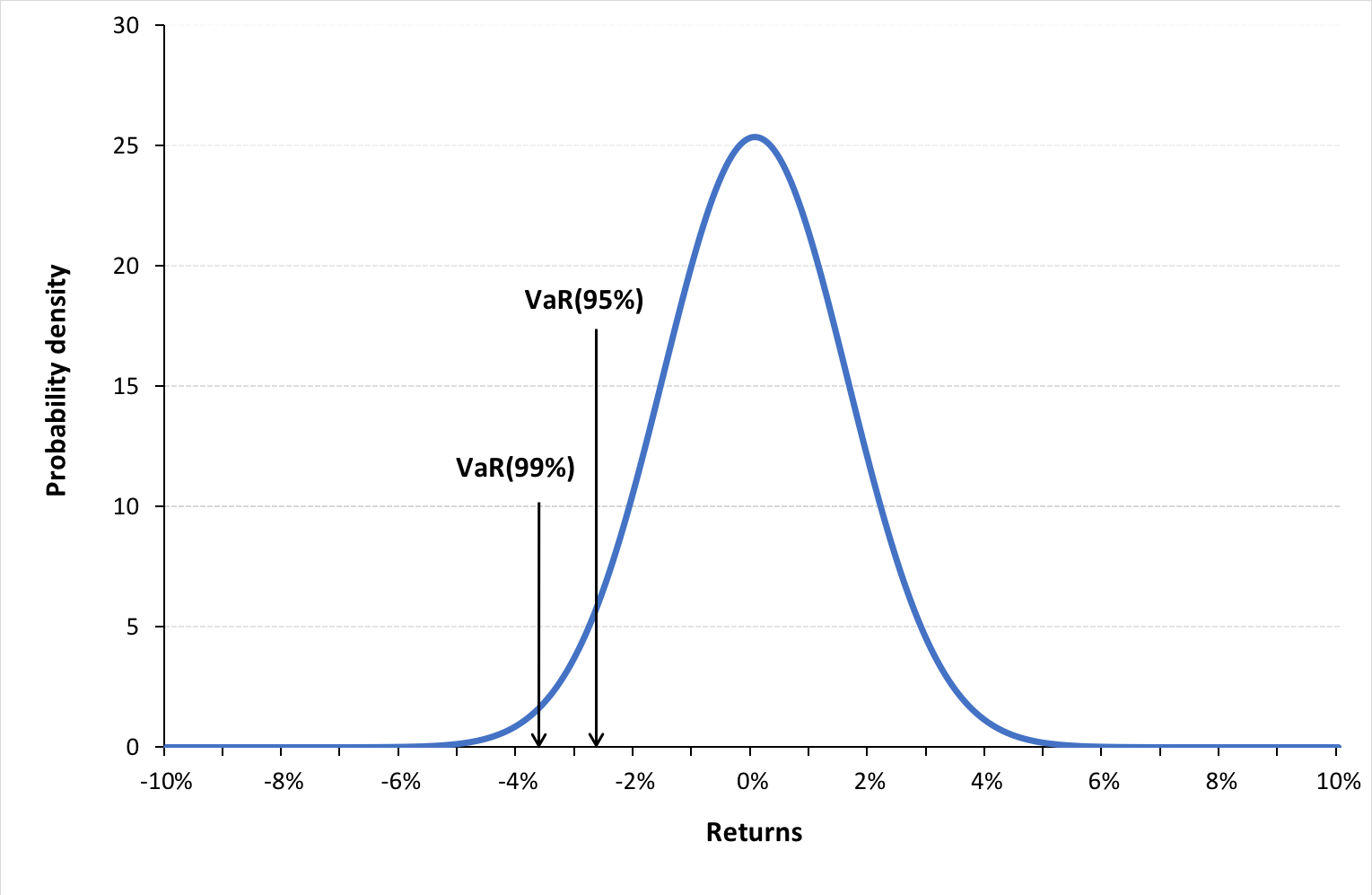
Source: computation by the author (data source: Bloomberg).
You can download below the Excel file for the VaR calculation with the variance-covariance method. The two parameters of the normal distribution (the mean and standard deviation) are estimated with historical data from the CAC 40 index.

VaR for a portfolio of assets
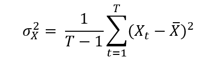
Consider a portfolio P with N assets. The first step is to compute the variance-covariance matrix. The variance of returns for asset X can be expressed as:
To measure how assets vary with each other, we calculate the covariance. The covariance between returns of two assets X and Y can be expressed as:
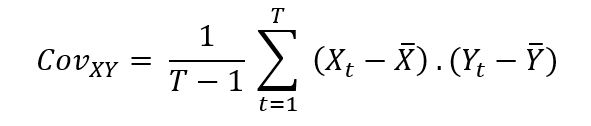
Where Xt and Yt are returns for asset X and Y on period [t-1, t].
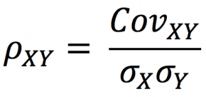
Next, we compute the correlation coefficients as:
We calculation the standard deviation of portfolio P with the following formula:
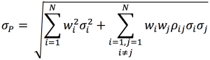
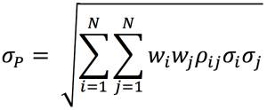
Where wi corresponds to portfolio weights of asset i.
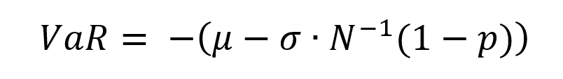
Now we can estimate the VaR of our portfolio as:
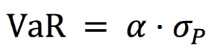
Where the parameter ɑ links the quantile of the normal distribution and the standard deviation: ɑ = 2.33 for p = 99% and ɑ = 1.65 for p = 95%.
Advantages and limitations of the variance-covariance method
Investors can estimate the probable loss value of their portfolios for different holding time periods and confidence levels. The variance–covariance approach helps us measure portfolio risk if returns are assumed to be distributed normally. However, the assumptions of return normality and constant covariances and correlations between assets in the portfolio may not hold true in real life.
Related posts on the SimTrade blog
▶ Jayati WALIA Quantitative Risk Management
▶ Jayati WALIA Value at Risk
▶ Jayati WALIA The historical method for VaR calculation
▶Jayati WALIA The Monte Carlo simulation method for VaR calculation
Useful resources
Jorion P. (2007) Value at Risk, Third Edition, Chapter 10 – VaR Methods, 274-276.
About the author
The article was written in December 2021 by Jayati WALIA (ESSEC Business School, Grande Ecole Program – Master in Management, 2019-2022).