

In this article, Saral BINDAL (Indian Institute of Technology Kharagpur, Metallurgical and Materials Engineering, 2024-2028 & Research assistant at ESSEC Business School) explains the expression “Mu versus Sigma” often used in asset management to study the impact of expected performance and risk on the safety of capital invested by individuals.
Introduction
In financial markets, performance over time is governed by three fundamental variables: the drift (μ), volatility (σ), and –perhaps most importantly– time (T). The drift represents the expected growth rate of the price and corresponds to the expected return of assets or portfolios. Volatility measures the uncertainty or risk associated with price fluctuations around this expected growth and corresponds to the standard deviation of returns. Time is not merely the mechanical passage of calendar time; it also embodies the investment horizon chosen by the investor, that is, the period over which risk is borne and returns are realized. The relationship between all variables reflects the trade-off between risk and return. Time, which is related to the investment horizon set by the investor, determines how both performance and risk accumulate. Together, these variables form the foundation of asset pricing to model the behavior of market price over time, and in fine the performance of the investor at their investment horizon.
Modeling asset prices with geometric Brownian motion (GBM)
Financial models commonly usually employ geometric Brownian motion (GBM) because it is a strictly non-negative stochastic process, making it well suited for modeling asset prices (a stock price must be positive under the limited lability rule). GBM provides a mathematically tractable and economically intuitive framework for describing the continuous-time evolution of asset prices under uncertainty.
Under GBM, the proportional change in an asset price is driven by a deterministic drift component and a random shock associated to volatility, represented by the stochastic differential equation:
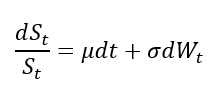
where:
- St = asset price at time t
- μ = drift (growth rate of the asset price)
- σ = volatility (standard deviation)
- dWt = infinitesimal increment of wiener process (N(0,dt))
This formulation leads to lognormally distributed prices and allows for closed-form expressions for expected values and confidence bounds, which are particularly useful in Monte Carlo simulations and risk analysis.
In practice, the continuous-time process is discretized (see Maruyama, 1955) to simulate price paths numerically. A more detailed discussion of the discrete GBM model and its implications is available in a separate post, which can be found here.
Figure 1 illustrates three simulated asset price paths generated under a geometric Brownian motion (GBM), sampled at monthly intervals (Δt = 1/12) over a 10-year horizon (T = 10). The expected price trajectory and the associated upper and lower bounds of the 66% confidence interval are shown alongside the simulations. The model assumes an annual drift (μ) of 8% and an annual volatility (σ) of 15%, with the initial asset price set at S0 = €100.
Figure 1. Monte Carlo simulated asset price paths under a Geometric Brownian Motion model.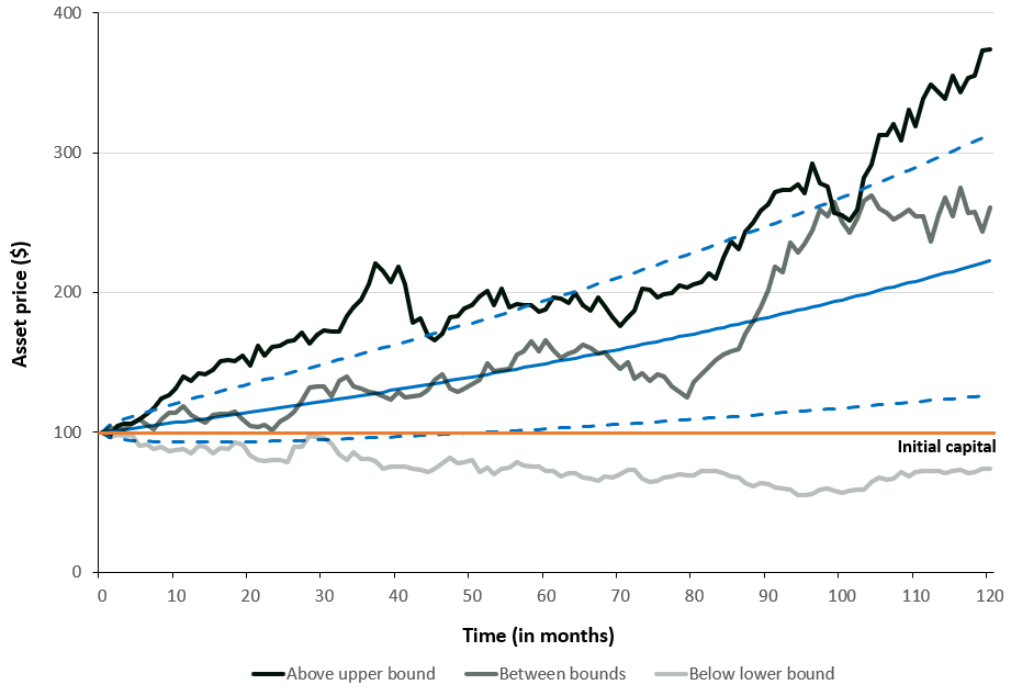
Source: computation by the author.
From Figure 1, the initial capital is set to $100, while the three simulated price paths illustrate alternative realizations of the asset’s stochastic evolution. These scenarios allow us to assess capital preservation over the investment horizon: when the terminal asset price remains above the initial capital level (either above the upper confidence bound or within the confidence band) the invested capital is preserved; conversely, when the price trajectory breaches the lower bound, the initial capital is eroded.
Time Scaling of Drift and Volatility: Mu versus Sigma
Under Brownian-based asset price models, the expected return grows linearly with time, while the dispersion around the mean increases proportionally to the square root of time. Accordingly, the μ and σ functions over time are given by:

In the formula above, the drift term must be replaced by μ-σ
The figure below illustrates the linear function μ(t) = t and the square-root function σ(t) = √t. These two functions are represented below for both μ and σ equal to 1.
Figure 2. Comparison of linear (t) and square-root (√t) time scaling.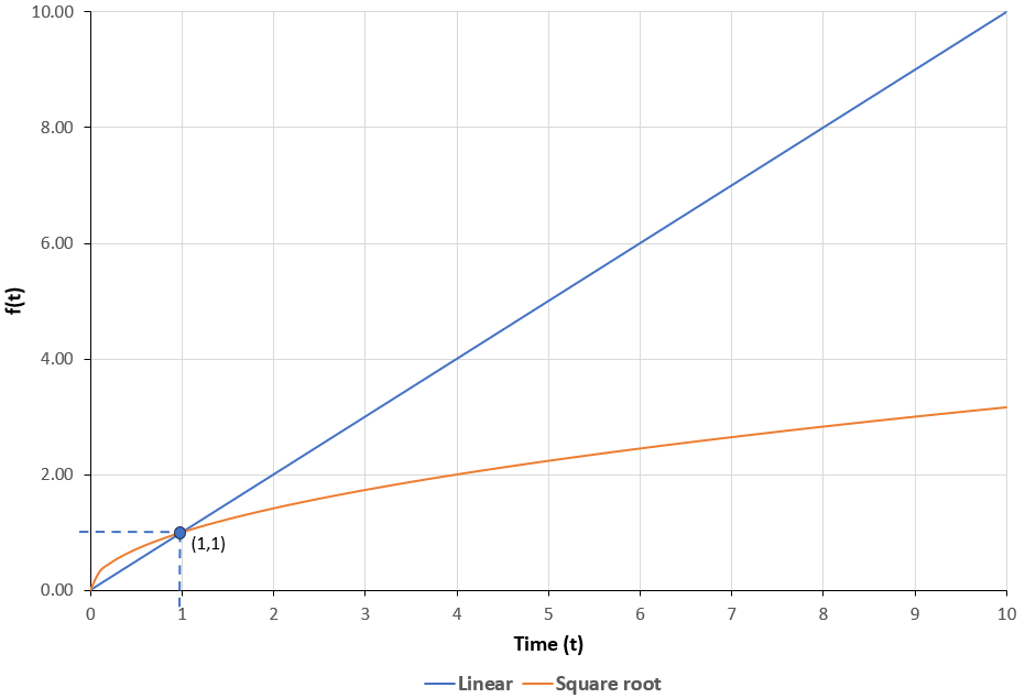
Source: computation by the author.
From Figure 2 above, we observe that at shorter time horizons (t < 1), the square-root function dominates the linear function, indicating that randomness (risk) has a stronger influence early on. At t = 1, both the functions are equal. For longer horizons (t > 1), the linear growth of the drift increasingly dominates the slower √t growth of volatility.
As discussed previously, the modelled prices also depend on the parameters μ (drift) and σ (volatility). This dependence is illustrated below through the functions μGBM(t) = μt and σGBM(t) = σ√t, with μ = μ-σ
Figure 3. Drift vs. Volatility as a function of time t.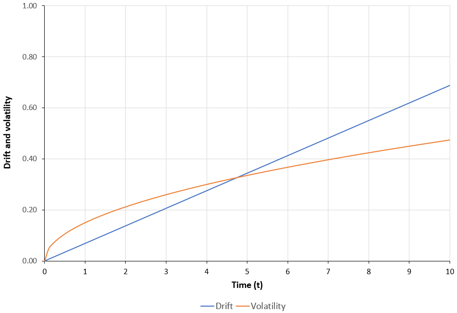
Source: computation by the author.
Capital safety
According to the safety-first principle (see Roy, 1952), the behavior of investors under uncertainty is driven by the tendency to minimize the probability of a disaster, defined as wealth or returns falling below a prespecified critical threshold d, rather than maximizing expected return. Formally, a disaster occurs when R < d, where R denotes expected returns. Typical disaster events include bankruptcy, severe capital loss, or failure to achieve a minimum acceptable outcome. The corresponding disaster probability is therefore given by:
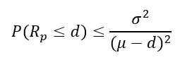
When returns are normally distributed, minimizing the disaster probability under the safety-first principle is equivalent to maximizing the Safety-First Ratio (SF Ratio), defined as:
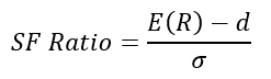
Where μ denotes the mean (expected return, E(R)) and σ the standard deviation (volatility), characterizing the distribution of returns of the asset under consideration.
When modelling asset prices or returns, realized outcomes may deviate from the mean, implying a strictly positive probability that the terminal price falls below any fixed reference level (for example, below $100 when 100 denotes the initial price).
Consequently, the lower bound of a given confidence interval is used to estimate the minimum return, or the disaster level (d), over a specified investment horizon. This lower bound can serve as a capital safety device, as capital safety is achieved by minimising the upper bound on the probability of disaster, or equivalently by maximising the SF Ratio.
In practice, such capital protection objectives are implemented through structured investment strategies such as structured products that combine fixed-income instruments with derivatives to ensure that the terminal payoff remains above a predefined threshold.
“Mu versus Sigma” and capital safety
Under the Geometric Brownian Motion (GBM), the theoretical expression for the lower bound of an asset’s logarithmic returns over time is given by:
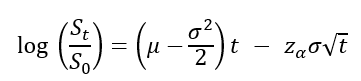
For the initial capital to be guaranteed at a given probability level, the lower confidence bound of returns must be positive at the investment horizon. A positive lower confidence bound implies that, with the specified confidence level, the terminal asset value does not fall below the initial investment, thereby providing probabilistic capital protection.
Condition for capital safety
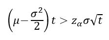
The evolution of lower bound over time depends on the following two cases:
Case 1: when μ − σ2/2 > 0
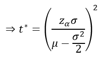
where t* is the minimum investment horizon for which the lower bound turns positive.
Case 2: when μ − σ2/2 ≤ 0
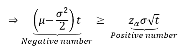
However, a non-positive quantity (zero or negative) cannot exceed a strictly positive one. As a result, the inequality can never be satisfied, and the critical time t^*does not exist.
Example: The S&P 500 index
Consider an investment in the S&P 500 index over a 10-year horizon, with an expected return (μ) of 8% and volatility (σ) of 15%. For a 66% confidence level, the critical investment horizon (t*) at which the lower confidence bound of terminal log-returns under a Geometric Brownian Motion (GBM) model becomes non-negative is given by:
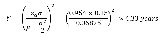
The table below shows the evolution of lower bound with time of investment, for returns on the above-mentioned investment,. From the table we can see that for time horizon less than 5, the lower bound is negative (ie no guarantee of initial cap) but after 5 years, the lower bound is positive hence gurantee of cap
The table below reports the evolution of the lower bound of returns as a function of the investment horizon. For short horizons (less than 4.33 years), the lower bound is negative, indicating that at the chosen confidence level there remains a non-zero probability of ending with a value below the initial capital. After 4.33 years the lower bound becomes positive, such that the terminal return is positive with the specified confidence level.
Table 1: Lower bound as function of investment horizon
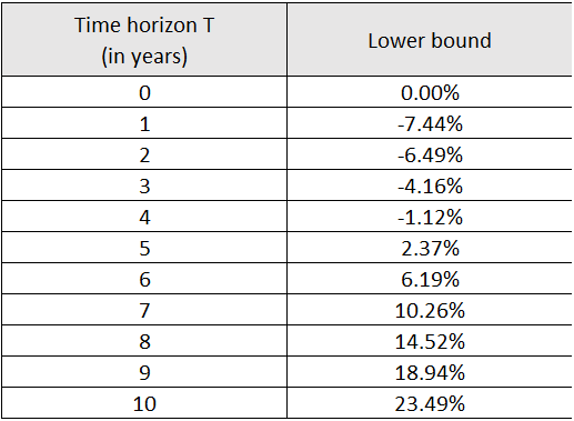
Thus, a minimum investment horizon of 4.33 years is required to guarantee the invested capital at the given probability.
Impact of the parameters on t*
Impact of μ on t*
As discussed above, the condition for t* to exist is (μ − σ2/2 > 0), therefore the value of μ at which t* exist is given by:
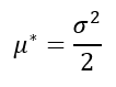
And the threshold value of μ for which the lower bound of log-returns first turns positive can be derived as follows:
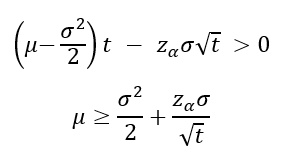
For the same S&P 500 investment example discussed above, with volatility (σ) fixed at 15% and the time to maturity set at 10 years, the value of μ* is calculated below.
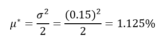
The table below reports the minimum investment horizon t* as a function of the drift parameter μ. For drift values below 1.125%, t* does not exist, reflecting the fact that the lower confidence bound of returns never becomes positive. Once the drift exceeds this threshold, t* becomes finite and decreases rapidly as μ increases. In particular, for μ ≥ 5%, the critical horizon falls below 10 years, indicating that capital protection can be achieved over the investment horizons considered, provided the expected growth rate is sufficiently high.
Table 2: t* as a function of μ
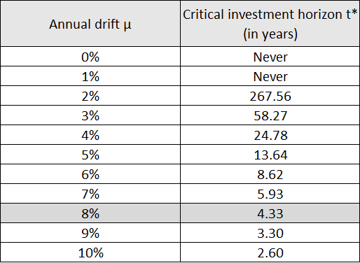
Therefore, under the GBM model, a drift of at least 5.56% is necessary for the lower confidence bound of returns to remain non-negative at a 10-year horizon.
Impact of σ on t*
As discussed above, the condition for t* to exist is (μ − σ2/2 > 0), therefore the value of σ at which t* exist is given by:
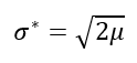
And the threshold value of σ for which the lower bound of log-returns first turns positive can be derived as follows:
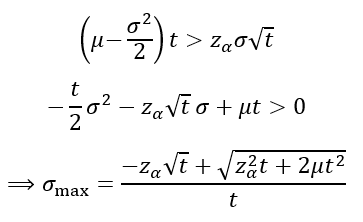
For the same S&P 500 investment example discussed above, with drift (μ) fixed at 8% and the time to maturity set at 10 years, the value of σ* is calculated below.

The table below reports the minimum investment horizon t* as a function of the volatility parameter &sigm;. For volatility values above 40%, t* does not exist, reflecting the fact that the lower confidence bound of returns never becomes positive. However, volatility values below this threshold, t* becomes finite and increases rapidly as σ increases. In particular, for σ ≥ 20%, the critical horizon exceeds 10 years, indicating that capital protection over a 10-year investment horizon is feasible only if volatility (risk) remains below 20%.
Table 3: t* as a function of σ
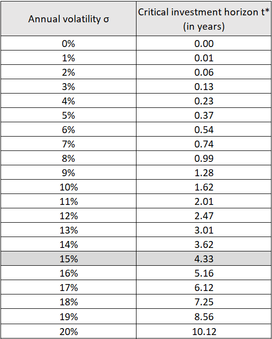
Therefore, under the GBM model, capital preservation over a 10-year horizon at the specified confidence level is feasible only if volatility does not exceed approximately 20%.
You can download the Excel file provided below to generate asset prices modeled using geometric Brownian motion and to illustrate the time scaling of drift and volatility, as well as the capital safety calculations discussed above.

Why should I be interested in this post?
Understanding how drift and volatility scale over time is central to the idea of capital safety and guarantee of capital. These concepts form the backbone of many structured products used by investors to protect their wealth, making them powerful tools for managing risk in uncertain markets.
Related posts on the SimTrade blog
▶ Saral BINDAL Historical Volatility
▶ Saral BINDAL Implied Volatility and Option Prices
▶ Jayati WALIA Brownian Motion in Finance
▶ Jayati WALIA Monte Carlo simulation method
Useful resources
Academic research
Bachelier L. (1900) Théorie de la spéculation. Annales scientifiques de l’École Normale Supérieure, 3e série, 17, 21–86.
de Haan L., Jansen D. W., Koedijk K. G., & de Vries C. G. (1994) Safety first portfolio selection, extreme value theory and heavy-tailed distributions. In: Extreme Value Theory and Applications, Springer, 471–487.
Kataoka S. (1963) A stochastic programming model. Econometrica, 31, 181–196.
Lawler G.F. (2006) Introduction to Stochastic Processes, 2nd Edition, Chapman & Hall/CRC, Chapter “Brownian Motion”, 201–224.
Maruyama G. (1955) Continuous Markov processes and stochastic equations. Rendiconti del Circolo Matematico di Palermo, 4, 48–90.
Roy A. D. (1952) Safety first and the holding of assets. Econometrica, 20, 431–449.
Samuelson P.A. (1965) Rational theory of warrant pricing. Industrial Management Review, 6(2), 13–39.
Telser L. G. (1955) Safety-first and hedging. Review of Economic Studies, 23, 1–16.
Wiener N. (1923) Differential-space. Journal of Mathematics and Physics, 2, 131–174.
About the author
The article was written in January 2026 by Saral BINDAL (Indian Institute of Technology Kharagpur, Metallurgical and Materials Engineering, 2024-2028 & Research assistant at ESSEC Business School).
Read all posts written by Saral BINDAL.
▶ Discover all articles written by Saral BINDAL