Modeling of the crude oil price

January 11, 2023 by Youssef LOURAOUI

Modeling of the crude oil price

In this article, Youssef LOURAOUI (Bayes Business School, MSc. Energy, Trade & Finance, 2021-2022) models the market price of the crude oil.

This article is structured as follows: we introduce the crude oil market. Then, we present the mathematical foundations of Geometric Brownian Motion (GBM) model. We use this model to simulate the price of crude oil.

The crude oil market

The crude oil market represents the physical (cash or spot) and paper (futures) market where buyers and sellers acquire oil.

Nowadays, the global economy is heavily reliant on fossil fuels such as crude oil, and the desire for these resources frequently causes political upheaval due to the fact that a few nations possess the greatest reservoirs. The price and profitability of crude oil are significantly impacted by supply and demand, like in any sector. The top oil producers in the world are the United States, Saudi Arabia, and Russia. With a production rate of 18.87 million barrels per day, the United States leads the list. Saudi Arabia, which will produce 10.84 million barrels per day in 2022 and own 17% of the world’s proved petroleum reserves, will come in second. Over 85% of its export revenue and 50% of its GDP are derived from the oil and gas industry. In 2022, Russia produced 10.77 million barrels every day. West Siberia and the Urals-Volga area contain the majority of the nation’s reserves. 10% of the oil produced worldwide comes from Russia.

Throughout the late nineteenth and early twentieth centuries, the United States was one of the world’s largest oil producers, and U.S. corporations developed the technology to convert oil into usable goods such as gasoline. U.S. oil output declined significantly throughout the middle and latter decades of the 20th century, and the country began to import energy. Nonetheless, crude oil net imports in 2021 were at their second-lowest yearly level since 1985. Its principal supplier was the Organization of the Petroleum Exporting Countries (OPEC), created in 1960, which consisted of the world’s largest (by volume) holders of crude oil and natural gas reserves.

As a result, the OPEC nations wielded considerable economic power in regulating supply, and hence price, of oil in the late twentieth century. In the early twenty-first century, the advent of new technology—particularly hydro-fracturing, or fracking—created a second U.S. energy boom, significantly reducing OPEC’s prominence and influence.

Oil spot contracts and futures contracts are the two forms of oil contracts that investors can exchange. To the individual investor, oil can be a speculative asset, a portfolio diversifier, or a hedge for existing positions.

Spot contract

The spot contract price indicates the current market price for oil, while the futures contract price shows the price that buyers are ready to pay for oil on a delivery date established in the future.

Most commodity contracts bought and sold on the spot market take effect immediately: money is exchanged, and the purchaser accepts delivery of the commodities. In the case of oil, the desire for immediate delivery vs future delivery is limited, owing to the practicalities of delivering oil.

Futures contract

An oil futures contract is an agreement to buy or sell a specified number of barrels of oil at a predetermined price on a predetermined date. When futures are acquired, a deal is struck between buyer and seller and secured by a margin payment equal to a percentage of the contract’s entire value. The futures price is no guarantee that oil will be at that price on that date in the future market. It is just the price that oil buyers and sellers anticipate at the time. The exact price of oil on that date is determined by a variety of factors impacting the supply and demand. Futures contracts are more frequently employed by traders and investors because investors do not intend to take any delivery of commodities at all.

End-users of oil buy on the market to lock in a price; investors buy futures to speculate on what the price will be in the future, and they earn if they estimate correctly. They typically liquidate or roll over their futures assets before having to take delivery. There are two major oil contracts that are closely observed by oil market participants: 1) West Texas Intermediate (WTI) crude, which trades on the New York Mercantile Exchange, serves as the North American oil futures benchmark (NYMEX); 2) North Sea Brent Crude, which trades on the Intercontinental Exchange, is the benchmark throughout Europe, Africa, and the Middle East (ICE). While the two contracts move in tandem, WTI is more sensitive to American economic developments, while Brent is more sensitive to those in other countries.

Mathematical foundations of the Geometric Brownian Motion (GBM) model

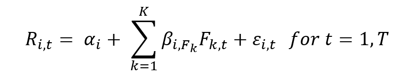
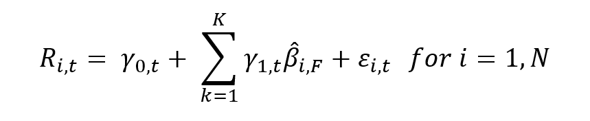
The concept of Brownian motion is associated with the contribution of Robert Brown (1828). More formally, the first works of Brown were used by the French mathematician Louis Bachelier (1900) applied to asset price forecast, which prepared the ground of modern quantitative finance. Price fluctuations observed over a short period, according to Bachelier’s theory, are independent of the current price as well as the historical behaviour of price movements. He deduced that the random behaviour of prices can be represented by a normal distribution by combining his assumptions with the Central Limit Theorem. This resulted in the development of the Random Walk Hypothesis, also known as the Random Walk Theory in modern finance. A random walk is a statistical phenomenon in which stock prices fluctuate at random. We implement a quantitative framework in a spreadsheet based on the Geometric Brownian Motion (GBM) model. Mathematically, we can derive the price of crude oil via the following model:

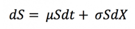
where dS represents the price change in continuous time dt, dX the Wiener process representing the random part, and Μdt the deterministic part.

The probability distribution function of the future price is a log-normal distribution when the price dynamics is described with a geometric Brownian motion.

Modelling crude oil market prices

Market prices

We downloaded a time series for WTI from June 2017 to June 2022. We picked this timeframe to assess the behavior of crude oil during two main market events that impacted its price: Covid-19 pandemic and the war in Ukraine.

The two main parameters to compute in order to implement the model are the (historical) average return and the (historical) volatility. We eliminated outliers (the negative price of oil) to clean the dataset and obtain better results. The historical average return is 11.99% (annual return) and the historical volatility is 59.29%. Figure 1 helps to capture the behavior of the WTI price over the period from June 2017 to June 2022.

Figure 1. Crude oil (WTI) price.
img_SimTrade_WTI_price
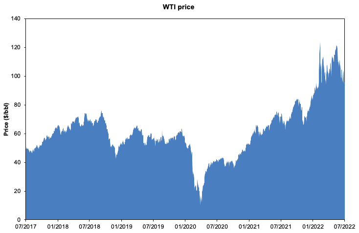
Source: computation by the author (data: Refinitiv Eikon).

Market returns

Figure 2 represents the returns of crude oil (WTI) over the period. We can clearly see that the impact of the Covid-19 pandemic had important implications for the negative returns in during the period covering early 2020.

Figure 2. Crude oil (WTI) return.
img_SimTrade_WTI_return
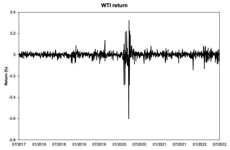
Source: computation by the author (data: Refinitiv Eikon).

We compute the returns using the log returns approach.

img_SimTrade_log_return_WTI

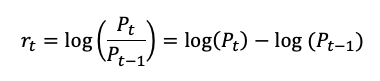
where P_t represents the closing price at time t.

Figure 3 captures the distribution of the crude oil (WTI) daily returns in a histogram. As seen in the plot, the returns are skewed towards the negative tail of the distribution and show some peaks in the center of the distribution. When analyzed in conjunction, we can infer that the crude oil daily returns doesn’t follow the normal distribution.

Figure 3. Histogram of crude oil (WTI) daily returns.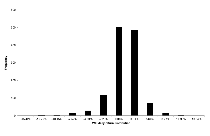 img_SimTrade_WTI_histogram Source: computation by the author (data: Refinitiv Eikon).

To have a better understanding of the crude oil behavior across the 1257 trading days retained for the period of analysis, it is interesting to run a statistical analysis of the four moments of the crude oil time series: the mean (average return), standard deviation (volatility), skewness (symmetry of the distribution), kurtosis (tail of the distribution). As captured by Table 1, crude oil performed positively over the period covered delivering a daily return equivalent to 0.05% (13.38% annualized return) for a daily degree of volatility equivalent to 3.74% (or 59.33% annualized). In terms of skewness, we can see that the distribution of crude oil return is highly negatively skewed, which implies that the negative tail of the distribution is longer than the right-hand tail (positive returns). Regarding the high positive kurtosis, we can conclude that the crude oil return distribution is more peaked with a narrow distribution around the center and show more tails than the normal distribution.

Table 1. Statistical moments of the crude oil (WTI) daily returns.
WTI statistical moment
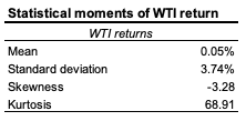
Source: computation by the author (data: Refinitiv Eikon).

Application: simulation of future prices for the crude oil market

Understanding the evolution of the price of crude oil can be significant for pricing purposes. Some models (such as the Black-Scholes option pricing model) rely heavily on a price input and can be sensitive to this parameter. Therefore, accurate price estimation is at the core of important pricing models and thus having a good estimate of spot and future price can have a significant impact in the accuracy of the pricing implemented profitability of the trade.

We implement this framework and use a Monte Carlo simulation of 25 iterations to capture the different path that the WTI price can take over a period of 24 months. Figure 4 captures the result of the model. We plot the simulations in a 3D-graph to grasp the shape of the variations in each maturity. As seen from Figure 4, price peaked at the longer end of the maturity at a level near the 250$/bbl. Overall the shape is bumpy, with some local spikes achieved throughout the whole sample and across all the maturities (Figure 4).

Figure 4. Geometric Brownian Motion (GBM) simulations for WTI.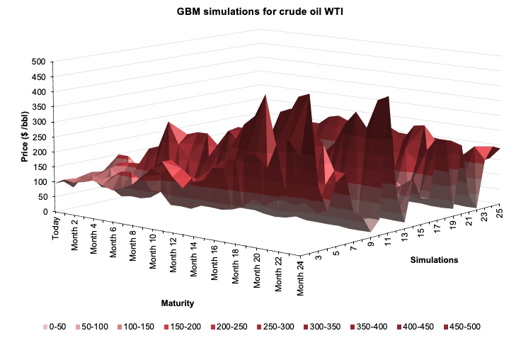 WTI GBM simulation Source: computation by the author (Data: Refinitiv Eikon).

You can find below the Excel spreadsheet that complements the explanations about of this article.

Useful resources

Academic research

Bachelier, Louis (1900). Théorie de la Spéculation, Annales Scientifique de l’École Normale Supérieure, 3e série, tome 17, 21-86.

Bashiri Behmiri, Niaz and Pires Manso, José Ramos, Crude Oil Price Forecasting Techniques: A Comprehensive Review of Literature (June 6, 2013). SSRN Reseach Journal.

Brown, Robert (1828), “A brief account of microscopical observations made on the particles contained in the pollen of plants” in Philosophical Magazine 4:161-173.

About the author

The article was written in January 2023 by Youssef LOURAOUI (Bayes Business School, MSc. Energy, Trade & Finance, 2021-2022).

Fama-MacBeth two-step regression method: the case of K risk factors

December 12, 2022 by Youssef LOURAOUI

Fama-MacBeth two-step regression method: the case of K risk factors

This article is structured as follows: we introduce the Fama-MacBeth two-step regression method. Then, we present the mathematical foundation that underpins their approach for K risk factors. We provide an illustration for the 3-factor mode developed by Fama and French (1993).

Introduction

Risk factors are frequently employed to explain asset returns in asset pricing theories. These risk factors may be macroeconomic (such as consumer inflation or unemployment) or microeconomic (such as firm size or various accounting and financial metrics of the firms). The Fama-MacBeth two-step regression approach found a practical way for measuring how correctly these risk factors explain asset or portfolio returns. The aim of the model is to determine the risk premium associated with the exposure to these risk factors.

The first step is to regress the return of every asset against one or more risk factors using a time-series approach. We obtain the return exposure to each factor called the “betas” or the “factor exposures” or the “factor loadings”.

The second step is to regress the returns of all assets against the asset betas obtained in Step 1 using a cross-section approach. We obtain the risk premium for each factor. Then, Fama and MacBeth assess the expected premium over time for a unit exposure to each risk factor by averaging these coefficients once for each element.

Mathematical foundations

We describe below the mathematical foundations for the Fama-MacBeth regression method for a K-factor application. In the analysis, we investigated the Fame-French three factor model in order to understand their significance as a fundamental driver of returns for investors under the Fama-MacBeth framework.

The model considers the following inputs:

The return of N assets denoted by R_i for asset i observed every day over the time period [0, T].
The risk factors denoted by F_k for k equal from 1 to K.

Step 1: time-series analysis of returns

For each asset i from 1 to N, we estimate the following linear regression model:

Fama-French time-series regression

From this model, we obtain the β_{i, Fk} which is the beta associated with the k^th risk factor.

Step 2: cross-sectional analysis of returns

For each period t from 1 to T, we estimate the following linear regression model:

Fama-French cross-sectional regression

Application: the Fama-French 3-Factor model

The Fama-French 3-factor model is an illustration of Fama-MacBeth two-step regression method in the case of K risk factors (K=3). The three factors are the market (MKT) factor, the small minus big (SMB) factor, and the high minus low (HML) factor. The SMB factor measures the difference in expected returns between small and big firms (in terms of market capitalization). The HML factor measures the difference in expected returns between value stocks and growth stock.

The model considers the following inputs:

The return of N assets denoted by R_i for asset i observed every day over the time period [0, T].
The risk factors denoted by F_MKT associated to the MKT risk factor, F_SMB associated to the MKT risk factor which measures the difference in expected returns between small and big firms (in terms of market capitalization) and F_HML associated to 𝐻𝑀𝐿 (“High Minus Low”) which measures the difference in expected returns between value stocks and growth stock

Step 1: time-series regression

img_SimTrade_Fama_French_time_series_regression

Step 2: cross-sectional regression

img_SimTrade_Fama_French_cross_sectional_regression

Figure 1 represents for a given period the cross-sectional regression of the return of all individual assets with respect to their estimated individual beta for the MKT factor.

Figure 1. Cross-sectional regression for the market factor.
Cross-section regression for the MKT factor Source: computation by the author.

Figure 2 represents for a given period the cross-sectional regression of the return of all individual assets with respect to their estimated individual beta for the SMB factor.

Figure 2. Cross-sectional regression for the SMB factor.
Cross-section regression for the SMB factor Source: computation by the author.

Figure 3 represents for a given period the cross-sectional regression of the return of all individual assets with respect to their estimated individual beta for the SMB factor.

Figure 3. Cross-sectional regression for the HML factor.
Cross-section regression for the HML factor Source: computation by the author.

Empirical study of the Fama-MacBeth regression

Fama-MacBeth seminal paper (1973) was based on an analysis of the market factor by assessing constructed portfolios of similar betas ranked by increasing values. This approach helped to overcome the shortcoming regarding the stability of the beta and correct for conditional heteroscedasticity derived from the computation of the betas for individual stocks. They performed a second time the cross-sectional regression of monthly portfolio returns based on equity betas to account for the dynamic nature of stock returns, which help to compute a robust standard error and assess if there is any heteroscedasticity in the regression. The conclusion of the seminal paper suggests that the beta is “dead”, in the sense that it cannot explain returns on its own (Fama and MacBeth, 1973).

Empirical study: Stock approach for a K-factor model

We collected a sample of 440 significant firms’ end-of-day stock prices in the US economy from January 3, 2012 to December 31, 2021. We calculated daily returns for each stock as well as the factor used in this analysis. We chose the S&P500 index to represent the market since it is an important worldwide stock benchmark that captures the US equities market.

Time-series regression

To assess the multi-factor regression, we used the Fama-MacBeth 3-factor model as the main factors assessed in this analysis. We regress the average returns for each stock against their factor betas. The first regression is statistically tested. This time-series regression is run on a subperiod of the whole period from January 03, 2012, to December 31, 2018. We use a t-statistic to explain the regression’s behavior. Because the p-value is in the rejection zone (less than the significance level of 5%), we can conclude that the factors can first explain an investor’s returns. However, as we will see later in the article, when we account for a second regression as proposed by Fama and MacBeth, the factors retained in this analysis are not capable of explaining the return on asset returns on its own. The stock approach produces statistically significant results in time-series regression at 10%, 5%, and even 1% significance levels. As shown in Table 1, the p-value is in the rejection range, indicating that the factors are statistically significant.

Table 1. Time-series regression t-statistic result.
Cross-section regression Source: computation by the author.

Cross-sectional regression

Over a second period from January 04, 2019, to December 31, 2021, we compute the dynamic regression of returns at each data point in time with respect to the betas computed in Step 1.

That being said, when the results are examined using cross-section regression, they are not statistically significant, as indicated by the p-value in Table 2. We are unable to reject the null hypothesis. The premium investors are evaluating cannot be explained solely by the factors assessed. This suggests that factors retained in the analysis fail to adequately explain the behavior of asset returns. These results are consistent with the Fama-MacBeth article (1973).

Table 2. Cross-section regression t-statistic result.
Source: computation by the author.

Excel file

You can find below the Excel spreadsheet that complements the explanations covered in this article.

Why should I be interested in this post?

Fama-MacBeth made a significant contribution to the field of econometrics. Their findings cleared the way for asset pricing theory to gain traction in academic literature. The Capital Asset Pricing Model (CAPM) is far too simplistic for a real-world scenario since the market factor is not the only source that drives returns; asset return is generated from a range of factors, each of which influences the overall return. This framework helps in capturing other sources of return.

Useful resources

Academic research

Brooks, C., 2019. Introductory Econometrics for Finance (4th ed.). Cambridge: Cambridge University Press. doi:10.1017/9781108524872

Fama, E. F., MacBeth, J. D., 1973. Risk, Return, and Equilibrium: Empirical Tests. Journal of Political Economy, 81(3), 607–636.

Roll R., 1977. A critique of the Asset Pricing Theory’s test, Part I: On Past and Potential Testability of the Theory. Journal of Financial Economics, 1, 129-176.

American Finance Association & Journal of Finance (2008) Masters of Finance: Eugene Fama (YouTube video)

About the author

The article was written in December 2022 by Youssef LOURAOUI (Bayes Business School, MSc. Energy, Trade & Finance, 2021-2022).

Fama-MacBeth regression method: the stock approach vs the portfolio approach

December 12, 2022 by Youssef LOURAOUI

Fama-MacBeth regression method: the stock approach vs the portfolio approach

In this article, Youssef LOURAOUI (Bayes Business School, MSc. Energy, Trade & Finance, 2021-2022) presents the Fama-MacBeth regression method used to test asset pricing models and addresses the difference when applying the regression method on individual stocks or portfolios composed of stocks with similar betas.

This article is structured as follow: we introduce the Fama-MacBeth testing method. Then, we present the mathematical foundation that underpins their approach. We conduct an empirical analysis on both the stock and the portfolio approach. We conclude with a discussion on econometric issues.

Introduction

As a reminder, the Fama-MacBeth regression method is composed on two steps: step 1 with a time-series regression and step 2 with a cross-section regression.

The first step is to regress the return of every stock against one or more risk factors using a time-series regression. We obtain the return exposure to each factor called the “betas” or the “factor exposures” or the “factor loadings”.

The second step is to regress the returns of all stocks against the asset betas obtained in the first step using a cross-section regression for different periods. We obtain the risk premium for each factor used to test the asset pricing model.

The implementation of this method can be done with individual stocks or with portfolios of stocks as proposed by Fama and MacBeth (1973). Their argument is the better stability of the beta when considering portfolios. In this article we illustrate the difference with the two implementations.

Fama and MacBeth (1973) implemented with individual stocks

We downloaded a sample of daily prices of stocks composing the S&P500 index over the period from January 03, 2012, to December 31, 2021 (we selected the stocks present from the beginning to the end of the period reducing our sample from 500 to 440 stocks). We computed daily returns for each stock and for the market factor retained in this study. To represent the market, we chose the S&P500 index, an important global stock benchmark capturing the US equity market.

The procedure to derive the Fama-MacBeth regression using the stock approach can be achieved as follow:

Step 1: time-series regression

We compute the beta of the stocks with respect to the market factor for the period covered (time-series regression). We estimate the beta of each stock related to the S&P500 index. The beta is computed as the slope of the linear regression of the stock return on the market return (S&P500 index return). This time-series regression is run on a subperiod of the whole period from January 03, 2012, to December 31, 2018.

Step 2: cross-sectional regression

Over a second period from January 04, 2019, to December 31, 2021, we compute the dynamic regression of returns at each data point in time with respect to the betas computed in Step 1.

With this procedure, we obtain a risk premium that would represent the relationship between the stock returns at each data point in time with their respective beta for the sample analyzed.

Test the statistical significance of the results obtained from the regression

Results in the time-series regression using the stock approach are statistically significant. As shown in Table 1, the p-value is in the rejection area, which implies that the factor that the market factor can be considered as a driver of return.

Table 1. Time-series regression t-statistic result.
img_SimTrade_Fama_MacBeth_cross_sectional_regression_stat_result Source: computation by the author.

However, when analyzed in the cross-section regression, the results are not statistically significant anymore. As shown in Table 2, the p-value is not in the rejection area. We cannot reject the null hypothesis (H0: non significance of the market factor). Market factor alone cannot explain the premium investors are considering.
This means that the market factor fails to explain properly the behavior of asset returns, which undermines the validity of the CAPM framework. These results are in line with the Fama-MacBeth paper (1973).

Table 2. Cross-section regression t-statistic result.
img_SimTrade_Fama_MacBeth_cross_sectional_regression_stat_result Source: computation by the author.

You can find below the Excel spreadsheet that complements the explanations covered in this part of the article (implementation of the Fama and MacBeth (1973) method with individual stocks).

Fama and MacBeth (1973) implemented with portfolios of stocks

The procedure to derive the Fama-MacBeth regression using the portfolio approach can be achieved as follow:

Step 1: time-series regression

We first compute the beta of the stocks with respect to the market factor for the period covered (time-series regression). We estimate the beta of each stock related to the S&P500 index. The beta is computed as the slope of the linear regression of the stock return on the market return (S&P500 index return). This time-series regression is run on a subperiod of the whole period from January 03, 2012, to December 31, 2015. We build twenty portfolios based on stock betas ranked in ascending order. The betas of the portfolios are then estimated again on a subperiod from January 04, 2016, to December 31, 2018.

It is challenging to maintain beta stability over time. Fama-MacBeth aimed to remedy this shortcoming through its novel technique. However, some issues must be addressed. When betas are calculated using a monthly time series, the statistical noise in the time series is significantly reduced in comparison to shorter time frames (i.e., daily observation). When portfolio betas are constructed, the coefficient becomes considerably more stable than when individual betas are evaluated. This is due to the diversification impact that a portfolio can produce, which considerably reduces the amount of specific risk.

Step 2: cross-sectional regression

Over a second period from January 03, 2019, to December 31, 2021, we compute the dynamic regression of portfolio returns at each data point in time with respect to the betas computed in Step 1.

With this procedure, we obtain a risk premium that would represent the relationship between the portfolio returns at each data point in time with their respective beta for the sample analyzed.

Test the statistical significance of the results obtained from the regression

Results in the cross-section regression using the portfolio approach are not statistically significant. As captured in Table 3, the p-value is not in the rejection area, which implies that the factor is statistically insignificant and that the market factor cannot be considered as a driver of return.

Table 3. Cross-section regression with portfolio approach t-statistic result.
img_SimTrade_Fama_MacBeth_Portfolio_cross_sectional_regression_stat_result Source: computation by the author.

You can find below the Excel spreadsheet that complements the explanations covered in this part of the article (implementation of the Fama and MacBeth (1973) method with portfolios of stocks).

Econometric issues

Errors in data measurement

Because regression uses a sample instead of the entire population, a certain margin of error must be accounted for since the authors derive estimated betas for the sample.

Asset return heteroscedasticity

In econometrics, heteroscedasticity is an important concern since it results in unequal residual variance. This indicates that a time series exhibiting some heteroscedasticity has a non-constant variance, which renders forecasting ineffective because the time series will not revert to its long-run mean.

Asset return autocorrelation

Standard errors in Fama-MacBeth regressions are solely corrected for cross-sectional correlation. This method does not fix the standard errors for time-series autocorrelation. This is typically not a concern for stock trading, as daily and weekly holding periods have modest time-series autocorrelation, whereas autocorrelation is larger over long horizons. This suggests that Fama-MacBeth regression may not be applicable in many corporate finance contexts where project holding durations are typically lengthy.

Why should I be interested in this post?

Useful resources

Academic research

Brooks, C., 2019. Introductory Econometrics for Finance (4th ed.). Cambridge: Cambridge University Press. doi:10.1017/9781108524872

Fama, E. F., MacBeth, J. D., 1973. Risk, Return, and Equilibrium: Empirical Tests. Journal of Political Economy, 81(3), 607–636.

Roll R., 1977. A critique of the Asset Pricing Theory’s test, Part I: On Past and Potential Testability of the Theory. Journal of Financial Economics, 1, 129-176.

American Finance Association & Journal of Finance (2008) Masters of Finance: Eugene Fama (YouTube video)

About the author

The article was written in December 2022 by Youssef LOURAOUI (Bayes Business School, MSc. Energy, Trade & Finance, 2021-2022).

Fama-MacBeth regression method: Analysis of the market factor

December 12, 2022 by Youssef LOURAOUI

In this article, Youssef LOURAOUI (Bayes Business School, MSc. Energy, Trade & Finance, 2021-2022) presents the Fama-MacBeth two-step regression method used to test asset pricing models. The seminal paper by Fama and MacBeth (1973) was based on an investigation of the market factor by evaluating portfolios of stocks with similar betas. In this article I will elaborate on the methodology and assess the statistical significance of the market factor as a fundamental driver of return.

This article is structured as follow: we introduce the Fama-MacBeth testing method used in asset pricing. Then, we present the mathematical foundation that underpins their approach. I then apply the Fama-MacBeth to recent US stock market data. Finally, I expose the limitations of their approach and conclude to discuss the generalization of the original study to other risk factors.

Introduction

The two-step regression method proposed by Fama-MacBeth was originally used in asset pricing to test the Capital Asset Pricing Model (CAPM). In this model, there is only one risk factor determining the variability of returns: the market factor.

The first step is to regress the return of every asset against the risk factor using a time-series approach. We obtain the return exposure to the factor called the “beta” or the “factor exposure” or the “factor loading”.

The second step is to regress the returns of all assets against the asset betas obtained in Step 1 during a given time period using a cross-section approach. We obtain the risk premium associated with the market factor. Then, Fama and MacBeth (1973) assess the expected premium over time for a unit exposure to the risk factor by averaging these coefficients once for each element.

Mathematical foundations

We describe below the mathematical foundations for the Fama-MacBeth two-step regression method.

Step 1: time-series analysis of returns

The model considers the following inputs:

The return of N assets denoted by R_i for asset i observed over the time period [0, T].
The risk factor denoted by F for the market factor impacting the asset returns.

For each asset i (for i varying from 1 to N) we estimate the following time-series linear regression model:

Fama MacBeth time-series regression

From this model, we obtain the following coefficients: α_i and β_i which are specific to asset i.

Figure 1 represents for a given asset (Apple stocks) the regression of its return with respect to the S&P500 index return (representing the market factor in the CAPM). The slope of the regression line corresponds to the beta of the regression equation.

Figure 1. Step 1: time-series regression for a given asset (Apple stock and the S&P500 index).
Source: computation by the author.

Step 2: cross-sectional analysis of returns

For each period t (from t equal 1 to T), we estimate the following cross-section linear regression model:

Fama MacBeth cross-section regression

Figure 2 plots for a given period the cross-sectional returns and betas for a given point in time.

Figure 2 represents for a given period the regression of the return of all individual assets with respect to their estimated individual market beta.

Figure 2. Step 2: cross-section regression for a given time-period.

Source: computation by the author.

We average the gamma obtained for each data point. This is the way the Fama-MacBeth method is used to test asset pricing models.

Empirical study of the Fama-MacBeth regression

The seminal paper by Fama and MacBeth (1973) was based on an analysis of the market factor by assessing constructed portfolios of similar betas ranked by increasing values. This approach helped to overcome the shortcoming regarding the stability of the beta and correct for conditional heteroscedasticity derived from the computation of the betas for individual stocks. They performed a second time the cross-sectional regression of monthly portfolio returns based on equity betas to account for the dynamic nature of stock returns, which help to compute a robust standard error and assess if there is any heteroscedasticity in the regression. The conclusion of the seminal paper suggests that the beta is “dead”, in the sense that it cannot explain returns on its own (Fama and MacBeth, 1973).

Empirical study: Stock approach

We downloaded a sample of end-of-month stock prices of large firms in the US economy over the period from March 31, 2016, to March 31, 2022. We computed monthly returns. To represent the market, we chose the S&P500 index.

We then applied the Fama-MacBeth two-step regression method to test the market factor (CAPM).

Figure 3 depicts the computation of average returns and the betas and stock in the analysis.

Figure 3. Computation of average returns and betas of the stocks.
Source: computation by the author.

Figure 4 represents the first step of the Fama-MacBeth regression. We regress the average returns for each stock with their respective betas.

Figure 4. Step 1 of the regression: Time-series analysis of returns
Source: computation by the author.

The initial regression is statistically evaluated. To describe the behavior of the regression, we employ a t-statistic. Since the p-value is in the rejection area (less than the significance limit of 5 percent), we can deduce that the market factor can at first explain the returns of an investor. However, as we are going deal in the later in the article, when we account for a second regression as formulated by Fama and MacBeth (1973), the market factor is not capable of explaining on its own the return of asset returns.

Figure 5 represents Step 2 of the Fama-MacBeth regression, where we perform for a given data point a regression of all individual stock returns with their respective estimated market beta.

Figure 5. Step 2: cross-sectional analysis of return.
Source: computation by the author.

Figure 6 represents the hypothesis testing for the cross-sectional regression. From the results obtained, we can clearly see that the p-value is not in the rejection area (at a 5% significance level), hence we cannot reject the null hypothesis. This means that the market factor fails to explain properly the behavior of asset returns, which undermines the validity of the CAPM framework. These results are in line with Fama-MacBeth (1973).

Figure 6. Hypothesis testing of the cross-sectional regression.
Source: computation by the author.

Excel file for the Fama-MacBeth two-step regression method

You can find below the Excel spreadsheet that complements the explanations covered in this article to implement the Fama-MacBeth two-step regression method.

Limitations of the Fama-McBeth approach

Selection of the market index

For the CAPM to be valid, we need to determine if the market portfolio is in the Markowitz efficient curve. According to Roll (1977), the market portfolio is not observable because it cannot capture all the asset classes (human capital, art, and real estate among others). He then believes that the returns cannot be captured effectively and hence makes the market portfolio, not a reliable factor in determining its efficiency.

Furthermore, the coefficients estimated in the time-series regressions are sensitive to the market index chosen for the study. These shortcomings must be taken into account when assessing CAPM studies.

Stability of the coefficients

The beta of individual assets are not stable over time. Fama and MacBeth attempted to address this shortcoming by implementing an innovative approach.

When betas are computed using a monthly time-series, the statistical noise of the time series is considerably reduced as opposed to shorter time frames (i.e., daily observation).

Using portfolio betas makes the coefficient much more stable than using individual betas. This is due to the diversification effect that a portfolio can achieve, reducing considerably the amount of specific risk.

Conclusion

Why should I be interested in this post?

Useful resources

Academic research

Brooks, C., 2019. Introductory Econometrics for Finance (4th ed.). Cambridge: Cambridge University Press. doi:10.1017/9781108524872

Fama, E. F., MacBeth, J. D., 1973. Risk, Return, and Equilibrium: Empirical Tests. Journal of Political Economy, 81(3), 607–636.

Roll R., 1977. A critique of the Asset Pricing Theory’s test, Part I: On Past and Potential Testability of the Theory. Journal of Financial Economics, 1, 129-176.

American Finance Association & Journal of Finance (2008) Masters of Finance: Eugene Fama (YouTube video)

Business Analysis

NEDL. 2022. Fama-MacBeth regression explained: calculating risk premia (Excel). [online] Available at: [Accessed 29 May 2022].

About the author

The article was written in December 2022 by Youssef LOURAOUI (Bayes Business School, MSc. Energy, Trade & Finance, 2021-2022).

Fama-MacBeth two-step regression method

January 30, 2024July 2, 2022 by Youssef LOURAOUI

In this article, Youssef Louraoui (Bayes Business School, MSc. Energy, Trade & Finance, 2021-2022) presents the Fama-MacBeth two-step regression method used to test asset pricing models.

This article is structured as follow: we introduce the Fama-MacBeth testing method. Then, we present the mathematical foundation that underpins their approach. We conclude with a practical case study followed by a discussion on econometric issues.

Introduction

Risk factors are frequently employed to explain asset returns in asset pricing theories. These risk factors may be macroeconomic (such as consumer inflation or unemployment) or microeconomic (such as firm size or various accounting and financial metrics of the firms). The Fama-MacBeth two-step regression approach a practical way for measuring how correctly these risk factors explain asset or portfolio returns. The aim of the model is to determine the risk premium associated with the exposure to these risk factors.

Mathematical foundations

We describe below the mathematical foundations for the Fama-MacBeth two-step regression method.

Step 1: time-series analysis of returns

The model considers the following inputs:

The return of N assets denoted by R_i for asset i observed over the time period [0, T].
The risk factors denoted by F₁ for the market factor influencing the asset returns.

For each asset i from 1 to N, we estimate the following parameters:

From this model, we obtain a series of coefficients: α_i which is the risk premium for asset i and the β_{i, F₁ associated to the market risk factor.}

Figure 1 represents for a given asset the regression of a return with respect to the market factor (as in the CAPM). The slope of the regression line corresponds to the market beta of the regression.

Figure 1 Time-series regression.
Source : computation by the author.

The econometric issues (estimation bias, heteroscedasticity, and autocorrelation) related to the model are discussed in more details in the econometric limitation section.

Step 2: cross-sectional analysis of returns

For each period t from 1 to T, we estimate the following linear regression model:

Figure 2 plots for a given period the cross-sectional returns and betas for a given point in time.

Figure 2 represents for a given period the regression of the return of all individual assets with respect to their estimated individual market beta.

Figure 2. Cross-sectional regression.
Time-series regression Source: computation by the author.

We average the gamma obtained for each data point. This is the way the Fama-MacBeth method is used to test asset pricing models.

Empirical study by Fama and MacBeth (1973)

Fama-MacBeth performed a second time the cross-sectional regression of monthly stock returns on the equity betas computed on the initial workings to account for the dynamic nature of stock returns, which help to compute a robust standard error to gauge the level of error and assess if there is any heteroscedasticity in the regression. The conclusion of the seminal paper suggests that the beta is “dead”, in the sense that it cannot explain returns on its own (Fama and MacBeth, 1973).

New empirical study

We then applied the Fama-MacBeth two-step regression method to test the market factor (CAPM).

Figure 3 depicts the computation of average returns and the betas and stock in the analysis.

Figure 3. Computation of average returns and betas of the stocks.
Source: computation by the author.

Figure 4 represents the first step of the Fama-MacBeth regression. We regress the average returns for each stock with their respective betas.

Figure 4. Step 1 of the regression: Time-series analysis of returns
Source: computation by the author.

The initial regression is statistically evaluated. To describe the behaviour of the regression, we employ a t-statistic. Since the p-value is in the rejection area (less than the significance limit of 5 percent), we can deduce that the market factor can at first explain the returns of an investor. However, as we are going deal in the later in the article, when we account for a second regression as formulated by Fama and MacBeth, the market factor is not capable of explaining on its own the return of asset returns.

Figure 5 represents Step 2 of the Fama-MacBeth regression, where we perform for a given data point a regression of all individual stock returns with their respective estimated market beta.

Figure 5. Step 2: cross-sectional analysis of return.
Source : computation by the author.

Figure 6 represents the hypothesis testing for the cross-sectional regression. From the results obtained, we can clearly see that the p-value is not in the rejection area (at a 5% significance level), hence we cannot reject the null hypothesis. This means that the market factor fails to explain properly the behaviour of asset returns, which undermines the validity of the CAPM framework. These results are in line with the Fama-MacBeth paper (1973).

Figure 6. Hypothesis testing of the cross-sectional regression.
Source: computation by the author.

Excel file for the Fama-MacBeth two-step regression method

You can find below the Excel spreadsheet that complements the explanations covered in this article to apply the Fama-MacBeth two-step regression method.

Econometric issues

Errors in data measurement

Because regression uses a sample instead of the entire population, a certain margin of error must be accounted for since the authors derive estimated betas for the sample.

Asset return heteroscedasticity

Asset return autocorrelation

Limitation of CAPM

Roll: selection of the appropriate market index

Furthermore, the coefficients are sensitive to the market index chosen for the study. These shortcomings must be taken into account when assessing other CAPM studies.

Fama-MacBeth: Stability of the coefficients

The stability of the beta across time is difficult. Fama-MacBeth attempted to address this shortcoming by implementing its innovative approach. However, some points need to be addressed:

When betas are computed using a monthly time series, the statistical noise of the time series is considerably reduced as opposed to shorter time frames (i.e., daily observation).

Constructing portfolio betas makes the coefficient much more stable than when assessing individual betas. This is due to the diversification effect that a portfolio can achieve, reducing considerably the amount of specific risk.

Why should I be interested in this post?

Useful resources

Academic research

Brooks, C., 2019. Introductory Econometrics for Finance (4th ed.). Cambridge: Cambridge University Press. doi:10.1017/9781108524872

Fama, E. F., MacBeth, J. D., 1973. Risk, Return, and Equilibrium: Empirical Tests. Journal of Political Economy, 81(3), 607–636.

Roll R., 1977. A critique of the Asset Pricing Theory’s test, Part I: On Past and Potential Testability of the Theory. Journal of Financial Economics, 1, 129-176.

American Finance Association & Journal of Finance (2008) Masters of Finance: Eugene Fama (YouTube video)

Business Analysis

NEDL. 2022. Fama-MacBeth regression explained: calculating risk premia (Excel). [online] Available at: [Accessed 29 May 2022].

About the author

The article was written in May 2022 by Youssef LOURAOUI (Bayes Business School, MSc. Energy, Trade & Finance, 2021-2022).

Modeling of the crude oil price

The crude oil market

Spot contract

Futures contract

Mathematical foundations of the Geometric Brownian Motion (GBM) model

Modelling crude oil market prices

Market prices

Market returns

Application: simulation of future prices for the crude oil market

Related posts on the SimTrade blog

Useful resources

Academic research

About the author

Fama-MacBeth two-step regression method: the case of K risk factors

Introduction

Mathematical foundations

Step 1: time-series analysis of returns

Step 2: cross-sectional analysis of returns

Application: the Fama-French 3-Factor model

Empirical study of the Fama-MacBeth regression

Empirical study: Stock approach for a K-factor model

Time-series regression

Cross-sectional regression

Excel file

Why should I be interested in this post?

Related posts on the SimTrade blog

Useful resources

Academic research

About the author

Fama-MacBeth regression method: the stock approach vs the portfolio approach

Introduction

Fama and MacBeth (1973) implemented with individual stocks

Step 1: time-series regression

Step 2: cross-sectional regression

Test the statistical significance of the results obtained from the regression

Fama and MacBeth (1973) implemented with portfolios of stocks

Step 1: time-series regression

Step 2: cross-sectional regression

Test the statistical significance of the results obtained from the regression

Econometric issues

Errors in data measurement

Asset return heteroscedasticity

Asset return autocorrelation

Why should I be interested in this post?

Related posts on the SimTrade blog

Useful resources

Academic research

About the author

Introduction

Mathematical foundations

Step 1: time-series analysis of returns

Step 2: cross-sectional analysis of returns

Empirical study of the Fama-MacBeth regression

Empirical study: Stock approach

Excel file for the Fama-MacBeth two-step regression method

Limitations of the Fama-McBeth approach

Selection of the market index

Stability of the coefficients

Conclusion

Why should I be interested in this post?

Related posts on the SimTrade blog

Useful resources

Academic research

Business Analysis

About the author

Introduction

Mathematical foundations

Step 1: time-series analysis of returns

Step 2: cross-sectional analysis of returns

Empirical study by Fama and MacBeth (1973)

New empirical study

Excel file for the Fama-MacBeth two-step regression method

Econometric issues

Errors in data measurement

Asset return heteroscedasticity

Asset return autocorrelation

Limitation of CAPM

Roll: selection of the appropriate market index

Fama-MacBeth: Stability of the coefficients

Why should I be interested in this post?