

In this article, Saral BINDAL (Indian Institute of Technology Kharagpur, Metallurgical and Materials Engineering, 2024-2028 & Research assistant at ESSEC Business School) analyzes the various shapes of volatility curves observed in financial markets and explains how they reveal market participants’ beliefs about future asset price distributions as implied by option prices.
Introduction
In financial markets characterized by uncertainty, volatility is a fundamental factor shaping the dynamics of the prices of financial instruments. Implied volatility stands out as a key metric as a forward-looking measure that captures the market’s expectations of future price fluctuations, as reflected in current market prices of options.
Implied volatility is inherently a two-dimensional object, as it is indexed by strike K and maturity T. The collection of these implied volatilities across all strikes and maturities constitutes the volatility surface. Under the Black–Scholes–Merton (BSM) framework, volatility is assumed to be constant across strikes and maturities, in which case the volatility surface would degenerate into a flat plane. Empirically, however, the volatility surface is highly structured and varies significantly across both strike and maturity.
Accordingly, this post focuses on implied volatility curves across moneyness for a fixed maturity (i.e. cross-sections of the volatility surface), examining their canonical shapes, economic interpretation, and the insights they reveal about market beliefs and risk preferences.
Option pricing
Option pricing aims to determine the fair value of options (calls and puts). One of the most widely used frameworks for this purpose is the Black–Scholes–Merton (BSM) model, which expresses the option value as a function of five key inputs: the underlying asset price S, the strike price K, time to maturity T, the risk-free interest rate r, and volatility σ. Given these parameters, the model yields the theoretical value of the option under specific market assumptions. The details of the BSM option pricing formulas along with variable definitions can be found in the article Black-Scholes-Merton option pricing model.
Implied volatility
In the Black–Scholes–Merton (BSM) model, volatility is an unobservable parameter, representing the expected future variability of the underlying asset over the option’s remaining life. In practice, implied volatility is obtained by inverting the BSM pricing formula (using numerical methods such as the Newton–Raphson algorithm) to find the specific volatility that equates the BSM theoretical price to the observed market price. The details for the mathematical process of calculation of implied volatility can be found in Implied Volatility and Option Prices.
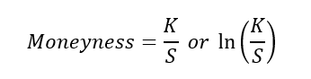
Moneyness
Moneyness describes the relative position of an option’s strike price K with respect to the current underlying asset price S. It indicates whether the option would have a positive intrinsic value if exercised at the current moment. Moneyness is typically parameterized using ratios such as K/S or its logarithmic transform.
In practice, moneyness classifies an option based on its intrinsic value. An option is said to be in-the-money (ITM) if it has positive intrinsic value, at-the-money (ATM) if its intrinsic value is zero, and out-of-the-money (OTM) if its intrinsic value is zero and immediate exercise would not be optimal. In terms of the relationship between the underlying asset price (S) and the strike price (K), a call option is ITM when S > K, ATM when S = K, and OTM when S < K. Conversely, a put option is ITM when S < K, ATM when S = K, and OTM when S > K.
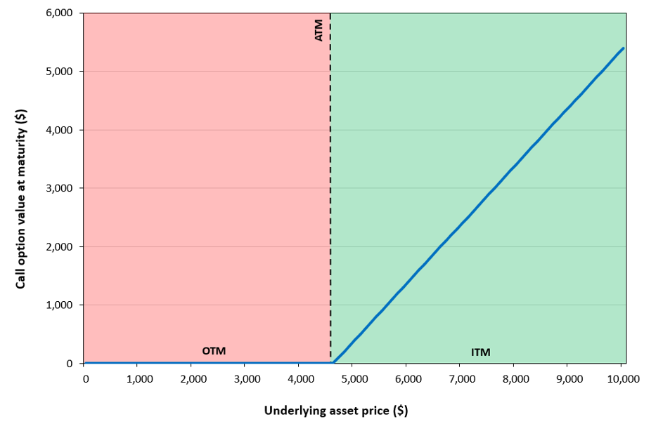
The payoff, that is the cash flow realized upon exercising the option at maturity T, is given for call and put options by:
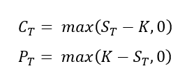
where ST is the underlying asset price at the time the option is exercised.
Figure 1 below illustrates the payoff of a call option, that is the call option value at maturity as a function of its underlying asset price. The call option’s strike price is assumed to be equal to $4,600. For an underlying price of $3,000, the call option is out-of-the-money (OTM); for a price of $4,600, the call option is at-the-money (ATM); and for a price of $7,000, the call option is in-the-money (ITM) and worth $2,400.
Figure 1. Payoff for a call option and its moneyness (OTM, ATM and ITM)
Source: computation by the author.
Similarly, Figure 2 below illustrates the payoff of a put option, that is the put option value at maturity as a function of its underlying asset price. The put option’s strike price is assumed to be equal to $4,600. For an underlying price of $3,000, the put option is in-the-money (ITM) and worth $1,600; for a price of $4,600, the put option is at-the-money (ATM); and for a price of $7,000, the put option is out-of-the-money (OTM).
Figure 2. Payoff for a put option and its moneyness (OTM, ATM and ITM)
Source: computation by the author.
Figure 3 below illustrates the temporal dynamics of moneyness for a European call option with a strike price of $4,600, showing how the option transitions between out-of-the-money, at-the-money, and in-the-money states as the underlying asset price moves relative to the strike over its lifetime.
Figure 3. Evolution of a call option moneyness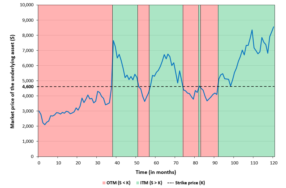
Source: computation by the author.
Similarly, Figure 4 below illustrates the temporal dynamics of moneyness for a European put option with a strike price of $4,600, showing how the option transitions between out-of-the-money, at-the-money, and in-the-money states as the underlying asset price moves relative to the strike over its lifetime.
Figure 4. Evolution of a put option moneyness 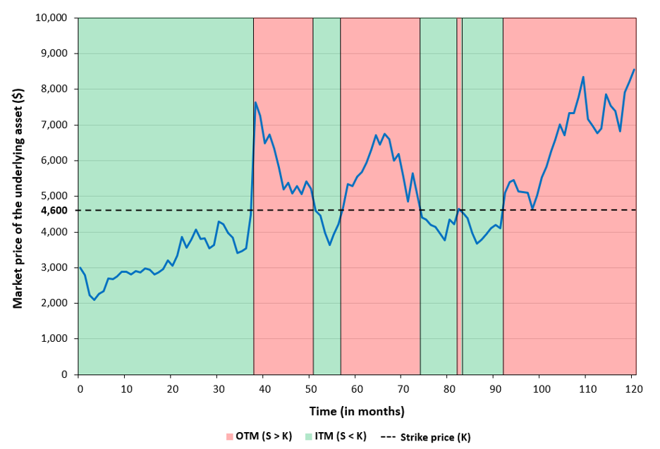
Source: computation by the author.
You can download the Excel file below for the computation of moneyness of call and put options as discussed in the above figures.

Empirical observation: implied volatility depends on moneyness
Smiles and smirks
Volatility curves refer to plots of implied volatility across different strikes for options with the same maturity. Two distinct shapes are commonly observed: the “volatility smile” and the “volatility smirk”.
A volatility smile is a symmetric pattern commonly observed in options markets. For a given underlying asset and expiration date, it is defined as the mapping of option strike prices to their Black–Scholes–Merton implied volatilities. The term “smile” refers to the distinctive shape of the curve: implied volatility is lowest near the at-the-money (ATM) strike and rises for both lower in-the-money (ITM) strikes and higher out-of-the-money (OTM) strikes.
A volatility smirk (also called skew) is an asymmetric pattern in the implied volatility curve and is mainly observed in the equity markets. It is characterized by high implied volatilities at lower strikes and progressively lower implied volatilities as the strike increases, resulting in a downward-sloping profile. This shape reflects the uneven distribution of implied volatility across strikes and stands in contrast to the more symmetric volatility smile observed in other markets.
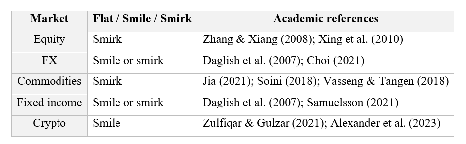
Stylized facts about the implied volatility curve across markets
Stylized facts characterizing implied volatility curves are persistent and statistically robust empirical regularities observed across financial markets. Below, I discuss the key stylized facts for major asset classes, including equities, foreign exchange, interest rates, commodities, and cryptocurrencies.
Equity market: For major equity indices, the implied volatility curve at a given maturity is typically a negatively sloped smirk: IV is highest for out of the money puts and declines as the strike moves up, rather than forming a symmetric smile (Zhang & Xiang, 2008). This left skew is persistent across maturities and provides useful signals at the individual stock level, where steeper smirks (higher OTM put vs ATM IV) forecast lower subsequent returns, consistent with markets pricing crash risk into downside options (Xing, Zhang & Zhao, 2010).
FX market: For foreign currency options, implied volatility curves most often display a U shaped smile: IV is lowest near at the money and higher for deep in or out of the money strikes, especially for major FX pairs (Daglish, Hull & Suo, 2007). The degree of symmetry depends on the correlation between the FX rate and its volatility, so near zero correlation gives a roughly symmetric smile, while non zero correlations generate skews or smirks that have been empirically documented in options on EUR/USD, GBP/USD and AUD/USD (Choi, 2021).
Commodity market: For commodity options, cross market evidence shows that implied volatility curves are generally negatively skewed with positive curvature, meaning they exhibit smirks rather than flat surfaces, with higher IV for downside strikes but still some smile like curvature (Jia, 2021). Studies on crude oil and related commodities also find pronounced smiles and smirks whose strength varies with fundamentals such as inventories and hedging pressure, reinforcing it is a core stylized fact in commodity derivatives (Soini, 2018; Vasseng & Tangen, 2018).
Fixed income market: Swaption markets display smiles and skews on their volatility curves: for a given expiry and tenor, implied volatility typically curves in moneyness and may tilt up or down depending on the correlation between the underlying rate and volatility (Daglish, Hull & Suo, 2007). Empirical work on the swaption volatility cube shows that simple one factor or SABR lifted constructions do not capture the full observed smile, indicating that a rich, strike and maturity dependent IV surface is itself a stylized feature of interest rate options (Samuelsson, 2021).
Crypto market: Bitcoin options exhibit a non flat implied volatility smile with a forward skew, and short dated options can reach very high levels of implied volatility, reflecting heavy tails and strong demand for certain strikes (Zulfiqar & Gulzar, 2021). Because of this forward skew, the paper concludes that Bitcoin options “belong to the commodity class of assets,” although later studies show that the Bitcoin smile can change shape across regimes and is often flatter than equity index skew (Alexander, Kapraun & Korovilas, 2023).
Summary of stylized facts about implied volatility
An Empirical Analysis of S&P 500 Implied Volatility
This section describes the data, methodology, and empirical considerations for the analysis of implied volatility of put options written on the S&P 500 index. We begin by highlighting a classical challenge in cross-sectional option data: asynchronous trading.
Asynchronous trading and measurement error
In empirical option pricing, the non-synchronous observation of option prices and the underlying asset price generates measurement errors in implied volatility estimation, as the building of the volatility curve based on an option pricing model relies on option prices with the underlying price observed at the same point of time.
Formally, let the option price C be observed at time tc, while the underlying asset price S is observed at time ts with ts ≠ tc. The observed option price therefore satisfies
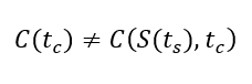
Since the option price at time tc depends on the latent spot price S(tc), rather than the asynchronously observed price S(ts), this mismatch introduces measurement error in the underlying price variable and implied volatility at the end.
Various standard filters including no-arbitrage, liquidity, moneyness, maturity, and implied-volatility sanity checks are typically applied to mitigate errors-in-variables arising from asynchronous observations of option prices and their underlying assets.
Example: options on the S&P 500 index
Consider the following sample of option data written on the S&P 500 index. Data can be obtained from FirstRate Data.
Figure 5 below illustrates the volatility smirk (or skew) for an option chain (a series of option prices for the same maturity) written on the S&P 500 index traded on 3rd July 2023 with time to maturity of 2 days after filtering it out from the above data.
Figure 5. Volatility smirk for put option prices on the S&P 500 index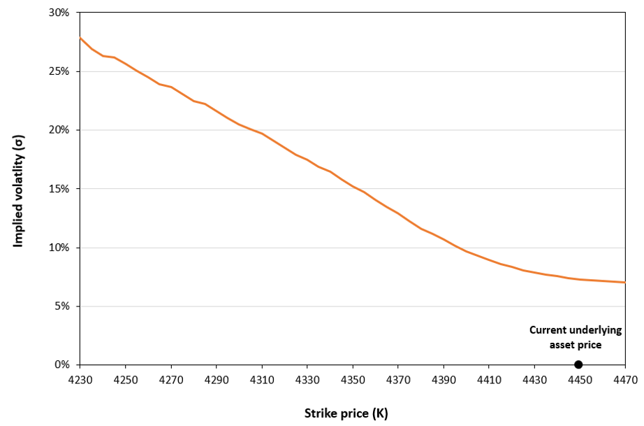
Source: computation by the author.
You can download the Excel file below to compute the volatility curve for put options on the S&P 500 index.
Economic Insights
This section explains how the shape of the implied volatility curve reveals key economic forces in options markets, including demand for crash protection, leverage-driven volatility feedback effects, and the role of market frictions and limits to arbitrage.
Demand for crash protection:
Out-of-the-money put options serve as insurance against market crashes and hedge tail risk. Because this demand is persistent and largely one-sided, put options become expensive relative to their Black–Scholes-Merton values, resulting in elevated implied volatilities at low strikes. This excess pricing reflects the market’s willingness to pay a premium to insure against rare but severe losses.
Leverage and volatility feedback effects:
When equity prices fall, firms become more leveraged because the value of equity declines relative to debt. Higher leverage makes equity riskier, increasing expected future volatility. Anticipating this effect, markets assign higher implied volatility to downside scenarios than to upside moves. This endogenous feedback between price declines, leverage, and volatility naturally produces a negative volatility skew, even in the absence of crash-risk preferences.
Market frictions and limits to arbitrage:
In practice, option writers are subject to capital constraints, margin requirements, and exposure to jump and tail risk. These constraints limit their capacity to supply downside protection at low prices. As a result, downside options embed not only compensation for fundamental crash risk, but also a risk premium reflecting the balance-sheet costs and risk-bearing capacity of intermediaries. The observed volatility skew therefore arises endogenously from limits to arbitrage rather than purely from differences in underlying return distributions.
Conclusion
The dependence of implied volatility on moneyness is neither an anomaly nor a technical artifact. It reflects market expectations, risk preferences, and the perceived probability of extreme outcomes. For both pedagogical and investment applications, the implied volatility curve is a central tool for understanding how markets price tail and downside risk.
Why should I be interested in this post?
Understanding implied volatility and its relationship with moneyness extends beyond option pricing, offering insights into how markets perceive risk and assess the likelihood of extreme events. Patterns such as volatility smiles and skews reflect investor behavior, the demand for protection, and the asymmetric emphasis on potential losses over gains, providing a clearer view of both pricing anomalies and the economic forces that shape financial markets.
Related posts on the SimTrade blog
Option price modelling
▶ Jayati WALIA Brownian Motion in Finance
▶ Saral BINDAL Modeling Asset Prices in Financial Markets: Arithmetic and Geometric Brownian Motions
▶ Jayati WALIA Black-Scholes-Merton option pricing model
▶ Jayati WALIA Monte Carlo simulation method
Volatility
▶ Saral BINDAL Historical Volatility
▶ Saral BINDAL Implied Volatility and Option Prices
▶ Jayati WALIA Implied Volatlity
Useful resources
Academic research on Option pricing
Black, F., & Scholes, M. (1973). The pricing of options and corporate liabilities, Journal of Political Economy, 81(3), 637–654.
Hull J.C. (2015) Options, Futures, and Other Derivatives, Ninth Edition, Chapter 15 – The Black-Scholes-Merton model, 343-375.
Merton, R.C. (1973). Theory of rational option pricing, The Bell Journal of Economics and Management Science, 4(1), 141–183.
Academic research on Stylized facts
Alexander, C., Kapraun, J. & Korovilas, D. (2023) Delta hedging bitcoin options with a smile, Quantitative Finance, 23(5), 799–817.
Bakshi, G., Cao, C., & Chen, Z. (1997). Empirical performance of alternative option pricing models, The Journal of Finance, 52(5), 2003–2049.
Bates, D. S. (1991). The crash of ’87: Was it expected? The evidence from options markets, The Journal of Finance, 46(5), 1777–1819.
Bates, D. S. (2000). Post-’87 crash fears in the S&P 500 futures option market, Journal of Econometrics, 94(1–2), 181–238.
Choi, K. (2021) Foreign exchange rate volatility smiles and smirks, Applied Stochastic Models in Business and Industry, 37(3), 405–425.
Daglish, T., Hull, J. & Suo, W. (2007) Volatility surfaces: theory, rules of thumb, and empirical evidence, Quantitative Finance, 7(5), 507–524.
Jia, G. (2021) The implied volatility smirk of commodity options, Journal of Futures Markets, 41(1), 72–104.
Samuelsson, A. (2021) Empirical study of methods to complete the swaption volatility cube. Master’s thesis, Uppsala University.
Soini, E. (2018) Determinants of volatility smile: The case of crude oil options. Master’s thesis, University of Vaasa.
Xing, Y., Zhang, X. & Zhao, R. (2010) What does individual option volatility smirk tell us about future equity returns? Review of Financial Studies, 23(5), 1979–2017.
Zhang, J.E. & Xiang, Y. (2008) The implied volatility smirk, Quantitative Finance, 8(3), 263–284.
Zulfiqar, N. & Gulzar, S. (2021) Implied volatility estimation of bitcoin options and the stylized facts of option pricing, Financial Innovation, 7(1), 67.
About the author
The article was written in January 2026 by Saral BINDAL (Indian Institute of Technology Kharagpur, Metallurgical and Materials Engineering, 2024-2028 & Research assistant at ESSEC Business School).
▶ Discover all articles written by Saral BINDAL