
Fama-MacBeth two-step regression method: the case of K risk factors

In this article, Youssef LOURAOUI (Bayes Business School, MSc. Energy, Trade & Finance, 2021-2022) presents the Fama-MacBeth two-step regression method used to test asset pricing models in the case of K risk factors.
This article is structured as follows: we introduce the Fama-MacBeth two-step regression method. Then, we present the mathematical foundation that underpins their approach for K risk factors. We provide an illustration for the 3-factor mode developed by Fama and French (1993).
Introduction
Risk factors are frequently employed to explain asset returns in asset pricing theories. These risk factors may be macroeconomic (such as consumer inflation or unemployment) or microeconomic (such as firm size or various accounting and financial metrics of the firms). The Fama-MacBeth two-step regression approach found a practical way for measuring how correctly these risk factors explain asset or portfolio returns. The aim of the model is to determine the risk premium associated with the exposure to these risk factors.
The first step is to regress the return of every asset against one or more risk factors using a time-series approach. We obtain the return exposure to each factor called the “betas” or the “factor exposures” or the “factor loadings”.
The second step is to regress the returns of all assets against the asset betas obtained in Step 1 using a cross-section approach. We obtain the risk premium for each factor. Then, Fama and MacBeth assess the expected premium over time for a unit exposure to each risk factor by averaging these coefficients once for each element.
Mathematical foundations
We describe below the mathematical foundations for the Fama-MacBeth regression method for a K-factor application. In the analysis, we investigated the Fame-French three factor model in order to understand their significance as a fundamental driver of returns for investors under the Fama-MacBeth framework.
The model considers the following inputs:
- The return of N assets denoted by Ri for asset i observed every day over the time period [0, T].
- The risk factors denoted by Fk for k equal from 1 to K.
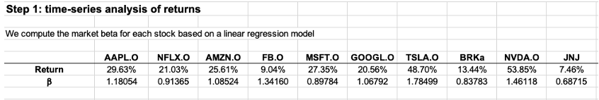
Step 1: time-series analysis of returns
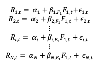
For each asset i from 1 to N, we estimate the following linear regression model:
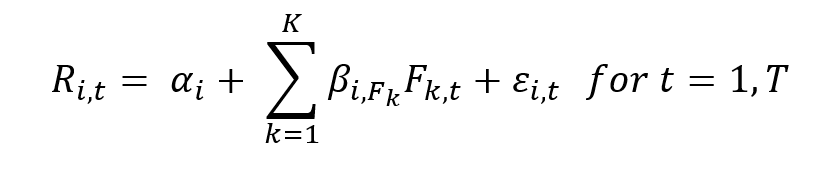
From this model, we obtain the βi, Fk which is the beta associated with the kth risk factor.
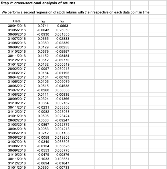
Step 2: cross-sectional analysis of returns
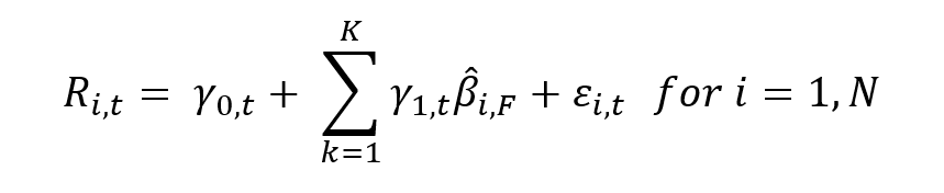
For each period t from 1 to T, we estimate the following linear regression model:
Application: the Fama-French 3-Factor model
The Fama-French 3-factor model is an illustration of Fama-MacBeth two-step regression method in the case of K risk factors (K=3). The three factors are the market (MKT) factor, the small minus big (SMB) factor, and the high minus low (HML) factor. The SMB factor measures the difference in expected returns between small and big firms (in terms of market capitalization). The HML factor measures the difference in expected returns between value stocks and growth stock.
The model considers the following inputs:
- The return of N assets denoted by Ri for asset i observed every day over the time period [0, T].
- The risk factors denoted by FMKT associated to the MKT risk factor, FSMB associated to the MKT risk factor which measures the difference in expected returns between small and big firms (in terms of market capitalization) and FHML associated to 𝐻𝑀𝐿 (“High Minus Low”) which measures the difference in expected returns between value stocks and growth stock
Step 1: time-series regression

Step 2: cross-sectional regression
![]()
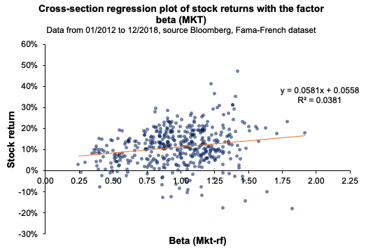
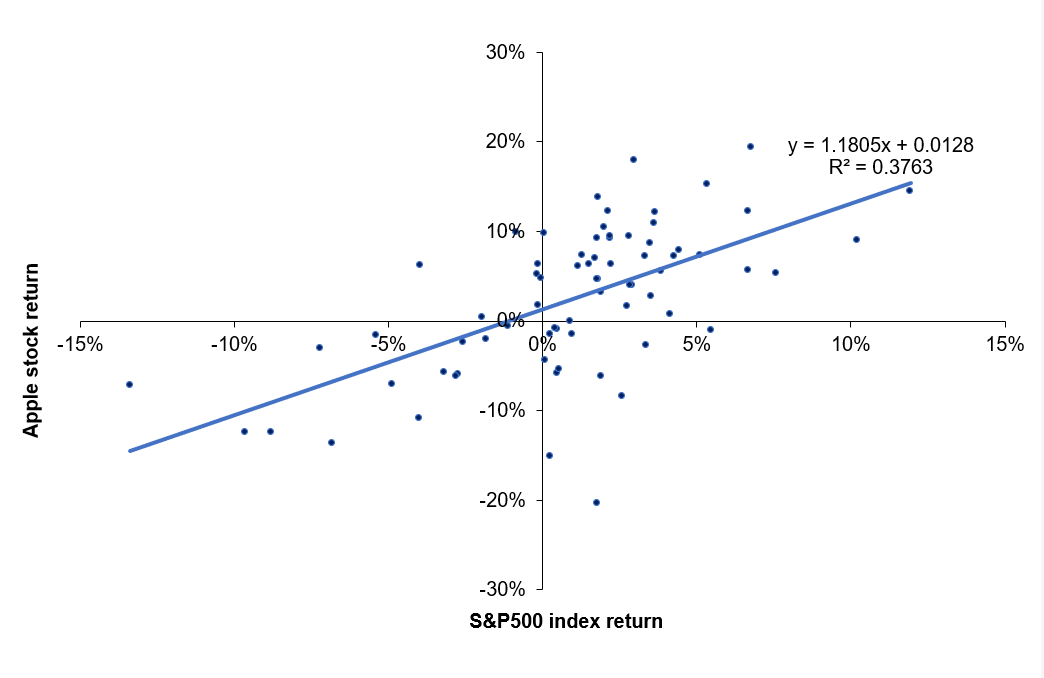
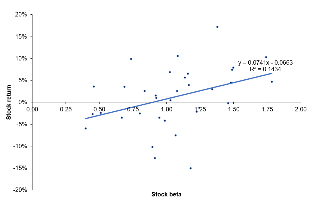
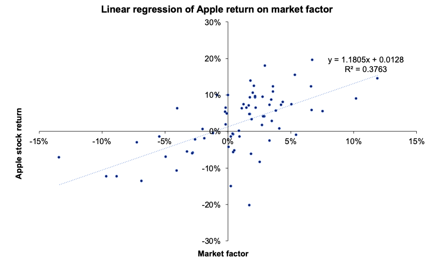
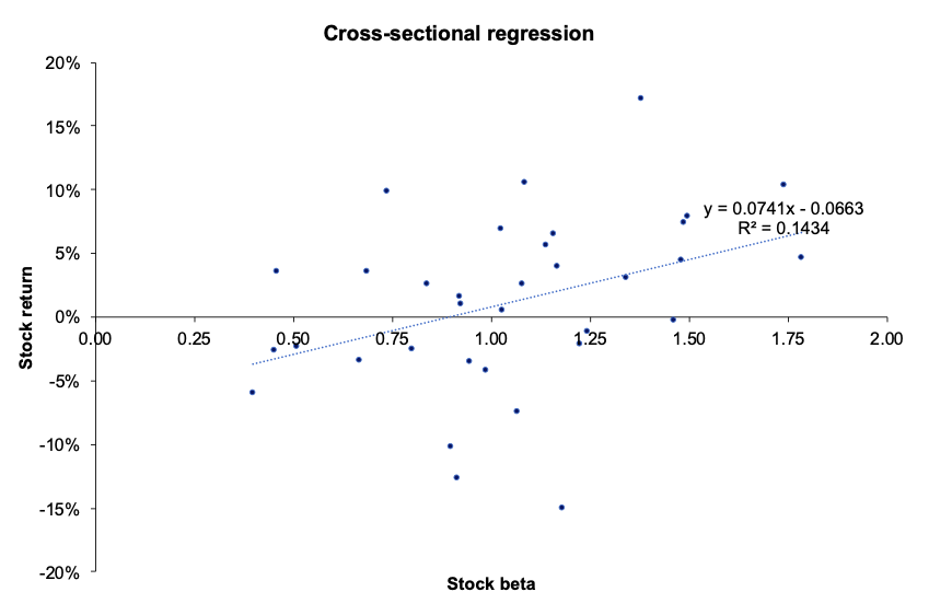
Figure 1 represents for a given period the cross-sectional regression of the return of all individual assets with respect to their estimated individual beta for the MKT factor.
Figure 1. Cross-sectional regression for the market factor.
 Source: computation by the author.
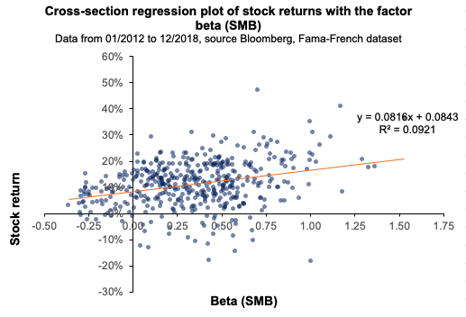
Figure 2 represents for a given period the cross-sectional regression of the return of all individual assets with respect to their estimated individual beta for the SMB factor.
Figure 2. Cross-sectional regression for the SMB factor.
 Source: computation by the author.
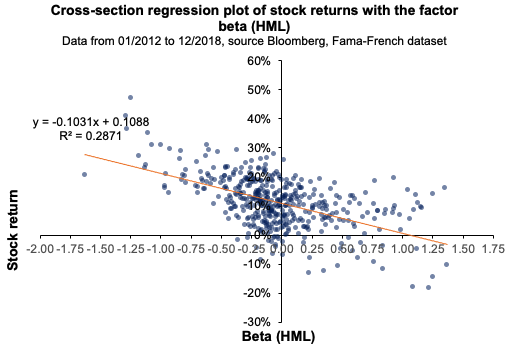
Figure 3 represents for a given period the cross-sectional regression of the return of all individual assets with respect to their estimated individual beta for the SMB factor.
Figure 3. Cross-sectional regression for the HML factor.
 Source: computation by the author.
Empirical study of the Fama-MacBeth regression
Fama-MacBeth seminal paper (1973) was based on an analysis of the market factor by assessing constructed portfolios of similar betas ranked by increasing values. This approach helped to overcome the shortcoming regarding the stability of the beta and correct for conditional heteroscedasticity derived from the computation of the betas for individual stocks. They performed a second time the cross-sectional regression of monthly portfolio returns based on equity betas to account for the dynamic nature of stock returns, which help to compute a robust standard error and assess if there is any heteroscedasticity in the regression. The conclusion of the seminal paper suggests that the beta is “dead”, in the sense that it cannot explain returns on its own (Fama and MacBeth, 1973).
Empirical study: Stock approach for a K-factor model
We collected a sample of 440 significant firms’ end-of-day stock prices in the US economy from January 3, 2012 to December 31, 2021. We calculated daily returns for each stock as well as the factor used in this analysis. We chose the S&P500 index to represent the market since it is an important worldwide stock benchmark that captures the US equities market.
Time-series regression
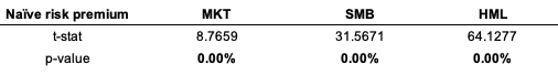
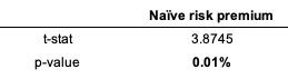
To assess the multi-factor regression, we used the Fama-MacBeth 3-factor model as the main factors assessed in this analysis. We regress the average returns for each stock against their factor betas. The first regression is statistically tested. This time-series regression is run on a subperiod of the whole period from January 03, 2012, to December 31, 2018. We use a t-statistic to explain the regression’s behavior. Because the p-value is in the rejection zone (less than the significance level of 5%), we can conclude that the factors can first explain an investor’s returns. However, as we will see later in the article, when we account for a second regression as proposed by Fama and MacBeth, the factors retained in this analysis are not capable of explaining the return on asset returns on its own. The stock approach produces statistically significant results in time-series regression at 10%, 5%, and even 1% significance levels. As shown in Table 1, the p-value is in the rejection range, indicating that the factors are statistically significant.
Table 1. Time-series regression t-statistic result.
 Source: computation by the author.
Cross-sectional regression
Over a second period from January 04, 2019, to December 31, 2021, we compute the dynamic regression of returns at each data point in time with respect to the betas computed in Step 1.
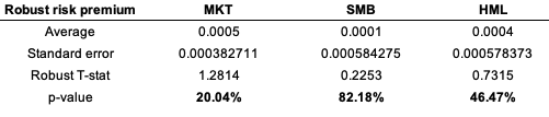
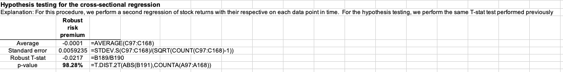
That being said, when the results are examined using cross-section regression, they are not statistically significant, as indicated by the p-value in Table 2. We are unable to reject the null hypothesis. The premium investors are evaluating cannot be explained solely by the factors assessed. This suggests that factors retained in the analysis fail to adequately explain the behavior of asset returns. These results are consistent with the Fama-MacBeth article (1973).
Table 2. Cross-section regression t-statistic result.
 Source: computation by the author.
Excel file
You can find below the Excel spreadsheet that complements the explanations covered in this article.

Why should I be interested in this post?
Fama-MacBeth made a significant contribution to the field of econometrics. Their findings cleared the way for asset pricing theory to gain traction in academic literature. The Capital Asset Pricing Model (CAPM) is far too simplistic for a real-world scenario since the market factor is not the only source that drives returns; asset return is generated from a range of factors, each of which influences the overall return. This framework helps in capturing other sources of return.
Related posts on the SimTrade blog
▶ Youssef LOURAOUI Fama-MacBeth regression method: stock and portfolio approach
▶ Youssef LOURAOUI Fama-MacBeth regression method: Analysis of the market factor
▶ Jayati WALIA Capital Asset Pricing Model (CAPM)
▶ Youssef LOURAOUI Security Market Line (SML)
▶ Youssef LOURAOUI Origin of factor investing
▶ Youssef LOURAOUI Factor Investing
Useful resources
Academic research
Brooks, C., 2019. Introductory Econometrics for Finance (4th ed.). Cambridge: Cambridge University Press. doi:10.1017/9781108524872
Fama, E. F., MacBeth, J. D., 1973. Risk, Return, and Equilibrium: Empirical Tests. Journal of Political Economy, 81(3), 607–636.
Roll R., 1977. A critique of the Asset Pricing Theory’s test, Part I: On Past and Potential Testability of the Theory. Journal of Financial Economics, 1, 129-176.
American Finance Association & Journal of Finance (2008) Masters of Finance: Eugene Fama (YouTube video)
About the author
The article was written in December 2022 by Youssef LOURAOUI (Bayes Business School, MSc. Energy, Trade & Finance, 2021-2022).
 Source: computation by the author.
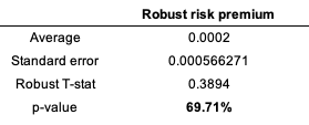 Source: computation by the author.
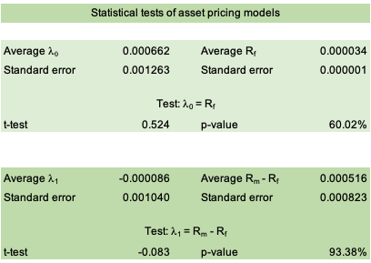 Source: computation by the author.
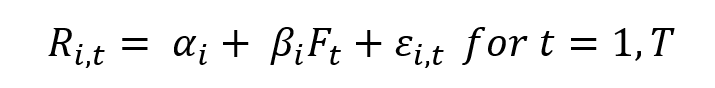
 Source: computation by the author.
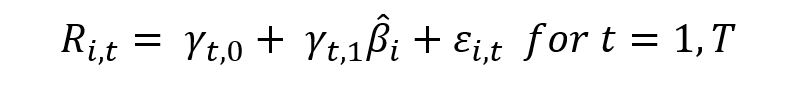
 Source : computation by the author.
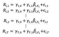
 Source: computation by the author.