Excel functions for mortgage

In this article, Liangyao TANG (ESSEC Business School, Master in Strategy & Management of International Business (SMIB), 2021-2022) explains the functions in Excel that are useful to study a mortgage. Mastery of Excel is an essential skill nowadays in financial analysis and modelling tasks. Proficiency in using Excel formulas can help analysts quickly process the data and build the models more concisely.
Mortgage
A mortgage is the type of loan used in real estate, vehicles, and other types of property purchasing activities. There are two parties in the mortgage contract: the borrower and the lender. The contract sets the terms and conditions about the principal amount, interest rate, interest type, payment period, maturity, and collaterals. The borrower is contracted to pay back the lender in a series of payments that contains part of the principal as well as the interests before the maturity date.
The mortgage is also subject to different terms according to the bank’s offers and macroeconomic cycle. There are two types of interest rates: the fixed-rate loan and the floating (variable) rate loan, in which the interest rate is a pre-determined rate (at the beginning of the period) and post-determined rate (at the end of the period).
Example of repayment schedule.
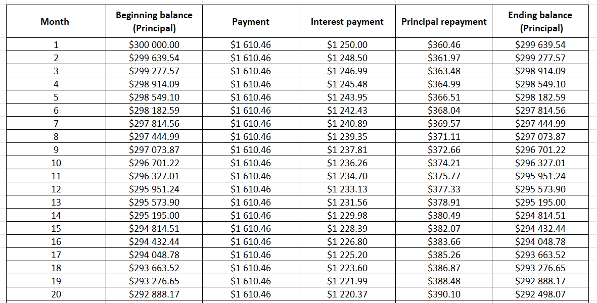
In this post, I will use the following example: a mortgage of $300,000 for property purchasing. The mortgage specifies a 5% fixed annual interest rate for 30 years, and the borrower should pay back the loan on a monthly basis. We can use Excel functions to calculate the periodic (monthly) payment and its two components, the principal repaid and the interests paid for a given period. The calculations are shown in the sample Excel file that you can download below.

PMT
The “PMT” (Payment) Excel function calculates the periodic mortgage payment.
The periodic repayment for a fixed-rate mortgage includes a portion of repayment to the principal and an interest payment. Since the mortgage has a given maturity date, the payment is calculated on a regular basis, for example, every month. All repayments are of equal amount throughout the loan period.
The mathematical formula for the periodic mortgage payment is:
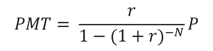
With the following notations:
- PMT: the payment
- P: the principal value
- r: the interest rate
- N: the total number of periods
The repayment schedule is a table which gives the periodic payment, and the principal repaid and the interests paid for a given period. It can be a large table. For example, the repayment schedule of a loan with 30 year maturity and monthly payment has 180 lines. In formal terms, the payment schedule would be:
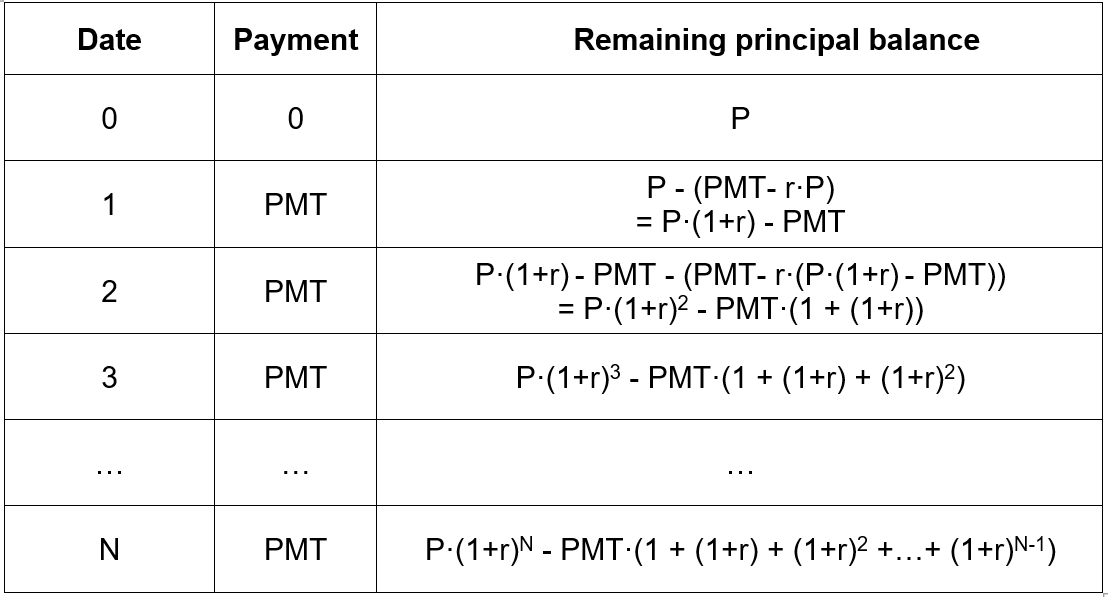
The repayment schedule shows the payment amount of each period, and the remaining principal balance after each payment. The ‘P’ represents the principal amount at the beginning of the mortgage, and the remaining principal is subjective to an (1+r) times interests at each period. The remaining principal is the principal balance from last period minus the current payment. Therefore for period 1, the remaining balance is equal to P(1+r), which is the principal with one year of interest, minus the PMT value, which is the payment of the current period.
The syntax for the Excel function to calculate the periodic payment is: PMT(rate, nper, pv, [fv], [type]).
With the following notations:
- PMT: the periodic payment of the loan
- Nper: the total number of periods of the loan
- PV : the principal (present value) of the loan
- [fv]: the future value of the loan (optional parameter). Default equal to 0
- [type]: when payments are due (optional parameter). 0 = end of period, 1 = beginning of period. Default is 0
The function is used explicitly in the case of a fixed interest rate to compute the (constant) periodic payment.
The PMT function will calculate the loan’s payment at a given level of interest rate, the number of periods, and the total value of the loan for principals at the beginning of the period (principal + interest).
When using the function, it is essential to always align the time unit of the interest rate and the unit of Nper. If the mortgage is compounding on a monthly basis, the number of periods should be the total number of months in the amortization, and the rate should be the monthly interest rate, which equals the annual rate divided by 12. . In the above example, the interest should be paid in a monthly basis, therefore the number of period (Nper) is equal to 12 month x 30 year = 360 periods. Since the annual interest rate is 5%, the monthly interest rate would equal to 5% divide by 12, which is 0.42% per month.
IPMT and PPMT
To supplement on the information about the monthly payment, we can also use the function IPMT and PPMT to calculate the principal repaid and the interest rate paid for a given period.
IPMT
IPMT is the Excel function that calculates the interest portion in each of the periodic payment.
The syntax of the Excel function to calculate the interest portion of the periodic payment is: IPMT(rate, per, nper, pv, [fv], [type]).
With the following notations:
- IPMT: interest payment
- rate: interest rate
- per: current period number
- nper: total number of periods
- pv: present value
- [fv]: the future value of the loan (optional parameter). Default equal to 0
- [type]: when payments are due (optional parameter). 0 = end of period, 1 = beginning of period. Default is 0
The rate refers to the periodic interest rate, while the “nper” refers to the total number of payment periods, and the “per” refers to the period for which we want to calculate the interest.
PPMT
PPMT is the Excel function that calculates the principal portion of a periodic payment.
The syntax of the Excel function to calculate the principal portion of a periodic payment is: PPMT(rate, per, nper, pv, [fv], [type]).
With the following notations:
- PPMT: principal payment
- rate: interest rate
- per: current period number
- nper: total number of periods
- pv: present value
- [fv]: the future value of the loan (optional parameter). Default equal to 0
- [type]: when payments are due (optional parameter). 0 = end of period, 1 = beginning of period. Default is 0
Those of the results should be consistent with the amortization schedule shown above. The principal repayment should equal to PMT per period minus the interest rate paid (IPMT).
RATE
Contrarily, if the user is given the periodic payment amount information and wants to find out about the interest rate used for the calculation, he/she can use the RATE function in Excel.
The syntax of the Excel function to calculate the rate is: RATE(nper, pmt, pv, [fv], [type], [guess]).
With the following notations:
- RATE: the interest rate
- nper: the total number of payment periods
- pmt: the constant periodic payment
- pv: the principal amount
- [fv]: the future value of the loan (optional parameter). Default equal to 0
- [type]: when payments are due (optional parameter). 0 = end of period, 1 = beginning of period. Default is 0
- [guess]: your guess on the rate (optional parameter). Default is 10%
The RATE Excel function will automatically calculate the interest rate per period. The time unit of the interest rate is aligned with the compounding period; for example, if the mortgage is compounding on a monthly basis, the RATE function also returns a monthly interest rate.
Example with an Excel file
The use of the Excel functions PMT, IPMT, PPMT and RATE is illustrated in the Excel file that you can download below.
Related posts on the SimTrade blog
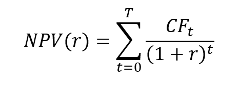
▶ Maite CARNICERO MARTINEZ How to compute the net present value of an investment in Excel
▶ William LONGIN How to compute the present value of an asset?
▶ Léopoldine FOUQUES The IRR, XIRR and MIRR functions in Excel
▶ Jérémy PAULEN The IRR function in Excel
Useful resources
Forbes What is a mortgage
Rocket mortgage Types of mortgage
Ramsey How Do Student Loans Work?
Prof. Longin’s website Echéancier d’un crédit (mortgage calculator in French)
About the author
The article was written in March 2022 by Liangyao TANG (ESSEC Business School, Master in Strategy & Management of International Business (SMIB), 2021-2022).