

In this article, Jayati WALIA (ESSEC Business School, Grande Ecole Program – Master in Management, 2019-2022) explains the Brownian motion and its applications in finance to model asset prices like stocks traded in financial markets.
Introduction
Stock price movements form a random pattern. The prices fluctuate everyday resulting from market forces like supply and demand, company valuation and earnings, and economic factors like inflation, liquidity, demographics of country and investors, political developments, etc. Market participants try to anticipate stock prices using all these factors and contribute to make price movements random by their trading activities as the financial and economics worlds are constantly changing.
What is a Brownian Motion?
The Brownian motion was first introduced by botanist Robert Brown who observed the random movement of pollen particles due to water molecules under a microscope. It was in the 1900s that the French mathematician Louis Bachelier applied the concept of Brownian motion to asset price behavior for the first time, and this led to Brownian motion becoming one of the most important fundamental of modern quantitative finance. In Bachelier’s theory, price fluctuations observed over a small time period are independent of the current price along with historical behavior of price movements. Combining his assumptions with the Central Limit Theorem, he also deduces that the random behavior of prices can be said to be represented by a normal distribution (Gaussian distribution).
This led to the development of the Random Walk Hypothesis or Random Walk Theory, as it is known today in modern finance. A random walk is a statistical phenomenon wherein stock prices move randomly.
When the time step of a random walk is made infinitesimally small, the random walk becomes a Brownian motion.
Standard Brownian Motion
In context of financial stochastic processes, the Brownian motion is also described as the Wiener Process that is a continuous stochastic process with normally distributed increments. Using the Wiener process notation, an asset price model in continuous time can be expressed as:
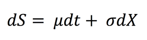
with dS being the change in asset price in continuous time dt. dX is the random variable from the normal distribution (N(0, 1) or Wiener process). σ is assumed to be constant and represents the price volatility considering the unexpected changes that can result from external effects. μdt together represents the deterministic return within the time interval with μ representing the growth rate of asset price or the ‘drift’.
When the market is modeled with a standard Brownian Motion, the probability distribution function of the future price is a normal distribution.
Geometric Brownian Motion
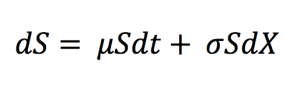
with dS being the change in asset price in continuous time dt. dX is the random variable from the normal distribution (N(0, 1) or Wiener process). σ is assumed to be constant and represents the price volatility considering the unexpected changes that can result from external effects. μdt together represents the deterministic return within the time interval with μ representing the growth rate of asset price or the ‘drift’.
When the market is modeled with a geometric Brownian Motion, the probability distribution function of the future price is a log-normal distribution.
Properties of a Brownian Motion
- Continuity: Brownian motion is the continuous time-limit of the discrete time random walk. It thus, has no discontinuities and is non-differential everywhere.
- Finite: The time increments are scaled with the square root of the times steps such that the Brownian motion is finite and non-zero always.
- Normality: Brownian motion is normally distributed with zero mean and non-zero standard deviation.
- Martingale and Markov Property: Martingale property states that the conditional expectation of the future value of a stochastic process depends on the current value, given information about previous events. The Markov property instead focusses on the ‘no memory’ theory that the expected future value of a stochastic process does not depend on any past values except the current value. Brownian motion follows both these properties.
Simulating Random Walks for Stock Prices
In quantitative finance, a random walk can be simulated programmatically through coding languages. This is essential because these simulations can be used to represent potential future prices of assets and securities and work out problems like derivatives pricing and portfolio risk evaluation.
A very popular mathematical technique of doing this is through the Monte Carlo simulations. In option pricing, the Monte Carlo simulation method is used to generate multiple random walks depicting the price movements of the underlying, each with an associated simulated payoff for the option. These payoffs are discounted back to the present value and the average of these discounted values is set as the option price. Similarly, it can be used for pricing other derivatives, but the Monte Carlo simulation method is more commonly used in portfolio and risk management.
For instance, consider Microsoft stock that has a current price of $258.65 with a growth trend of 55.2% and a volatility of 35.92%.
A plot of daily returns represented as a random normal distribution is:
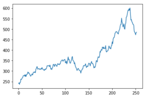
The above figure represents the simulated price path according to the Geometric Brownian motion for the Microsoft stock price. Similarly, a plot of 10 such simulations would be like this:
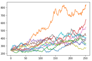
Thus, we can see that with just 10 simulations, the prices range from $100 to over $600. We can increase the number of simulations to expand the data set for analysis and use the results for derivatives pricing and many other financial applications.
Brownian motion and the efficient market hypothesis
If the market is efficient in the weak sense (as introduced by Fama (1970)), the current price incorporates all information contained in past prices and the best forecast of the future price is the current price. This is the case when the market price is modelled by a Brownian motion.
Related Posts
▶ Jayati WALIA Black-Scholes-Merton option pricing model
▶ Jayati WALIA Plain Vanilla Options
▶ Jayati WALIA Derivatives Market
▶ Modeling Asset Prices in Financial Markets: Arithmetic and Geometric Brownian Motions
Useful Resources
Academic articles
Fama E. (1970) Efficient Capital Markets: A Review of Theory and Empirical Work, Journal of Finance, 25, 383-417.
Fama E. (1991) Efficient Capital Markets: II Journal of Finance, 46, 1575-617.
Books
Malkiel B.G. (2020) A Random Walk Down Wall Street: The Time-tested Strategy for Successful Investing, WW Norton & Co.
Code
Python code for graphs and simulations
What is the random walk theory?
About the author
The article was written in August 2021 by Jayati WALIA (ESSEC Business School, Grande Ecole Program – Master in Management, 2019-2022).
2 thoughts on “Brownian Motion in Finance”
Comments are closed.