

In this article, Rishika YADAV (ESSEC Business School, Global Bachelor in Business Administration (GBBA), 2023–2027) explains the concept of risk-adjusted return, with a focus on the Sharpe ratio and complementary performance measures used in portfolio management.
Risk-adjusted return
Risk-adjusted return measures how much return an investment generates relative to the level of risk taken. This allows meaningful comparisons across portfolios and funds. For example, two portfolios may both generate a 12% return, but the one with lower volatility is superior because most investors are risk-averse — they prefer stable and predictable returns. A portfolio that achieves the same return with less risk provides higher utility to a risk-averse investor. In other words, it offers better compensation for the risk taken, which is precisely what risk-adjusted measures like the Sharpe Ratio capture.
The Sharpe Ratio
The Sharpe Ratio is the most widely used risk-adjusted performance measure. It standardizes excess return (return minus the risk-free rate) by total volatility and answers the question: how much additional return does an investor earn per unit of risk?
Sharpe Ratio = (E[RP] − Rf) / σP
where Rp = portfolio return, Rf = risk-free rate (e.g., T-bill yield), and σp = standard deviation of portfolio returns (volatility).
Interpretation
The Sharpe Ratio was developed by Nobel Laureate William F. Sharpe (1966) as a way to measure the excess return of an investment relative to its risk. A higher Sharpe ratio indicates better risk-adjusted performance.
- < 1 = sub-optimal
- 1–2 = acceptable to good
- 2–3 = very good
- > 3 = excellent (rarely achieved consistently)
In real financial markets, sustained Sharpe Ratios above 1.0 are uncommon. Over the past four decades, broad equity indices like the S&P 500 have averaged between 0.4 and 0.7, while balanced multi-asset portfolios often fall in the 0.6–0.9 range. Only a handful of hedge funds or quantitative strategies have achieved Sharpe ratios consistently above 1.0, and values exceeding 1.5 are exceptionally rare. Thus, while the Sharpe ratio is a useful comparative tool, the theoretical thresholds (e.g., >3 as “excellent”) are not typically observed in real markets.
Capital Allocation Line (CAL) and Capital Market Line (CML)
The Capital Allocation Line (CAL) represents the set of portfolios obtainable by combining a risk-free asset with a chosen risky portfolio P. It is a straight line in the (risk, expected return) plane: investors choose a point on the CAL according to their risk preference.
The equation of the CAL is:
E[RQ] = Rf + ((E[RP] − Rf) / σP) × σQ
where:
- E[Rp] = expected return of the combined portfolio
- Rf = risk-free rate
- E[RP] = expected return of risky portfolio P
- σP = standard deviation of P
- σQ = resulting standard deviation of the combined portfolio (proportional to weight in P)
The slope of the CAL equals the Sharpe ratio of portfolio P:
Slope(CAL) = (E[RP] − Rf) / σP = Sharpe(P)
The Capital Market Line (CML) is the CAL when the risky portfolio Q is the market portfolio (M). Under CAPM/Markowitz assumptions the market portfolio is the tangent (highest Sharpe) point on the efficient frontier and the CML is tangent to the efficient frontier at M.
The equation of the CML is:
E[RQ] = Rf + ((E[RM] − Rf) / σM) × σQ
where M denotes the market portfolio.
The slope of the CML, (E[RM] − Rf) / σM, is the Sharpe ratio of the market portfolio.
The link between the CAL, CML and Sharpe ratio is illustrated in the figure below.
Figure 1. Capital Allocation Line (CAL), Capital Market Line (CML) and the Sharpe ratio.
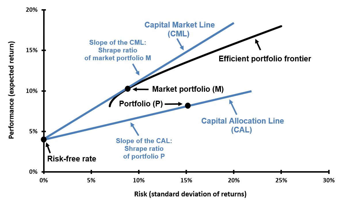
Source: computation by author.
Strengths of the Sharpe Ratio
- Simple and intuitive — easy to compute and interpret.
- Versatile — applicable across asset classes, funds, and portfolios.
- Balances reward and risk — combines excess return and volatility into a single metric.
Limitations of the Sharpe Ratio
- Assumes returns are approximately normally distributed — real returns often show skewness and fat tails.
- Penalizes upside and downside volatility equally — it does not distinguish harmful downside movements from beneficial upside.
- Sensitive to the chosen risk-free rate and the return measurement horizon (daily/monthly/annual).
Beyond Sharpe: Alternative measures
- Treynor Ratio — uses systematic risk (β) instead of total volatility: Treynor = (Rp − Rf) / βp. Best for well-diversified portfolios.
- Sortino Ratio — focuses only on downside deviation, so it penalizes harmful volatility (losses) but not upside variability.
- Jensen’s Alpha — α = Rp − [Rf + βp(Rm − Rf)]; measures manager skill relative to CAPM expectations.
- Information Ratio — active return (vs benchmark) divided by tracking error; useful for evaluating active managers.
Applications in portfolio management
Risk-adjusted metrics are used by asset managers to screen and rank funds, by institutional investors for capital allocation, and by analysts to determine whether outperformance is due to skill or increased risk exposure. When two funds have similar absolute returns, the one with the higher Sharpe Ratio is typically preferred.
Why should I be interested in this post?
Understanding the Sharpe Ratio and complementary risk-adjusted measures is essential for students interested in careers in asset management, equity research, or investment analysis. These tools help you evaluate performance meaningfully and make better investment decisions.
Related posts on the SimTrade blog
▶ Understanding Correlation and Portfolio Diversification
▶ Implementing the Markowitz Asset Allocation Model
▶ Markowitz and Modern Portfolio Theory
Useful resources
Jensen, M. (1968) The Performance of Mutual Funds in the Period 1945–1964, Journal of Finance, 23(2), 389–416.
Sharpe, W.F. (1966) Mutual Fund Performance, Journal of Business, 39(1), 119–138.
Sharpe, W.F. (1994) The Sharpe Ratio, Journal of Portfolio Management, 21(1), 49–58.Sortino, F. and Price, L. (1994) Performance Measurement in a Downside Risk Framework, Journal of Investing, 3(3), 59–64.
About the author
This article was written in October 2025 by Rishika YADAV (ESSEC Business School, Global Bachelor in Business Administration (GBBA), 2023–2027). Her academic interests lie in strategy, finance, and global industries, with a focus on the intersection of policy, innovation, and sustainable development.