

In this article, Jayati WALIA (ESSEC Business School, Grande Ecole – Master in Management, 2019-2022) presents linear regression.
Definition
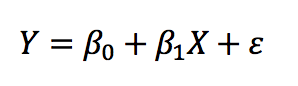
Linear regression is a basic and one of the commonly used type of predictive analysis. It attempts to devise the relationship between two variables by fitting a linear function to observed data. A simple linear regression line has an equation of the form:
Application in finance
For instance, consider Apple stock (AAPL). We can estimate the beta of the stock by creating a linear regression model with the dependent variable being AAPL returns and explanatory variable being the returns of an index (say S&P 500) over the same time period. The slope of the linear regression function is our beta.
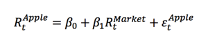
Figure 1 represents the return on the S&P 500 index (X axis) and the return on the Apple stock (Y axis), and the regression line given by the estimation of the linear regression above. The slope of the linear regression gives an estimate of the beta of the Apple stock.
Figure 1. Example of beta estimation for an Apple stock.
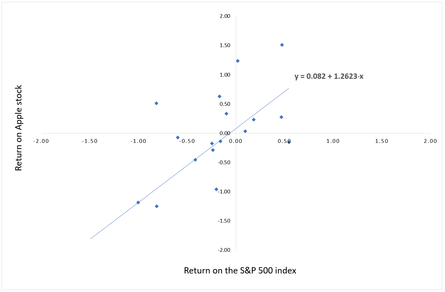
Source: computation by the author (Data: Apple).
Before attempting to fit a linear model to observed data, it is essential to determine some correlation between the variables of interest. If there appears to be no relation between the proposed independent/explanatory and dependent, then the linear regression model will probably not be of much use in the situation. A numerical measure of this relationship between two variables is known as correlation coefficient, which lies between -1 and 1 (1 indicating positively correlated, -1 indicating negatively correlated, and 0 indicating no correlation). A popularly used method to evaluate correlation among the variables is a scatter plot.
The overall idea of regression is to examine the variables that are significant predictors of the outcome variable, the way they impact the outcome variable and the accuracy of the prediction. Regression estimates are used to explain the relationship between one dependent variable and one or more independent variables and are widely applied to domains in business, finance, strategic analysis and academic study.
Assumptions in the linear regression model
The first step in the process of establishing a linear regression model for a particular data set is to make sure that the in consideration can actually be analyzed using linear regression. To do so, our data set must satisfy some assumptions that are essential for linear regression to give a valid and accurate result. These assumptions are explained below:
Continuity
The variables should be measured at a continuous level. For example, time, scores, prices, sales, etc.
Linearity
The variables in consideration must share a linear relationship. This can be observed using a scatterplot that can help identify a trend in the relationship of variables and evaluate whether it is linear or not.
No outliers in data set
An outlier is a data point whose outcome (or dependent) value is significantly different from the one observed from regression. It can be identified from the scatterplot of the date, wherein it lies far away from the regression line. Presence of outliers is not a good sign for a linear regression model.
Homoscedasticity
The data should satisfy the statistical concept of homoscedasticity according to which, the variances along the best-fit linear-regression line remain equal (or similar) for any value of explanatory variables. Scatterplots can help illustrate and verify this assumption
Normally-distributed residuals
The residuals (or errors) of the regression line are normally distributed with a mean of 0 and variance σ. This assumption can be illustrated through a histogram with a superimposed normal curve.
Ordinary Least Squares (OLS)
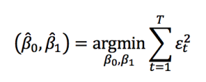
Once we have verified the assumptions for the data set and established the relevant variables, the next step is to estimate β0 and β1 which is done using the ordinary least squares method. Using OLS, we seek to minimize the sum of the squared residuals. That is, from the given data we calculate the distance from each data point to the regression line, square it, and calculate sum of all of the squared residuals(errors) together.
Thus, the optimization problem for finding β0 and β1 is given by:
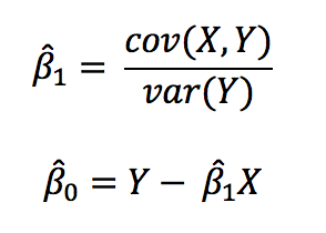
After computation, the optimal values for β0 and β1 are given by:
Using the OLS strategy, we can obtain the regression line from our model which is closest to the data points with minimum residuals. The Gauss-Markov theorem states that, in the class of conditionally unbiased linear estimators, the OLS estimators are considered as the Best Linear Unbiased Estimators (BLUE) of the real values of β0 and β1.
R-squared values
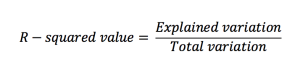
R-squared value of a simple linear regression model is the rate of the response variable variation. It is a statistical measure of how well the data set is fitted in the model and is also known as coefficient of determination. R-squared value lies between 0 and 100% and is evaluated as:
The greater is the value for R-squared, the better the model fits the data set and the more accurate is the predicted outcome.
Useful Resources
Related Posts
▶ Louraoui Y. Beta
About the author
The article was written in August 2021 by Jayati WALIA (ESSEC Business School, Grande Ecole – Master in Management, 2019-2022).
1 thought on “Linear Regression”
Comments are closed.