Understanding the Almgren-Chriss Model for Optimal Trade Execution

Bryan BOISLEVE

In this article, Bryan BOISLEVE (CentraleSupélec – ESSEC Business School, Data Science, 2023-2025) explains the Almgren-Chriss model, a fundamental framework in quantitative finance for optimal execution of large trading orders.

Introduction

Imagine you are a portfolio manager at a large asset management firm, and you need to sell 1 million shares of a stock. If you sell everything right now, you will significantly move the market price against yourself which comes with massive transaction costs. However, if you spread the trades over a too long a period, you expose yourself to the risk of adverse price movements due to market volatility. This dilemma between these two scenarios is one of the major optimal execution problems in finance.

The Almgren-Chriss model, developed by Robert Almgren and Neil Chriss in 2000, provides a mathematical framework to solve this problem. It has become an important model of algorithmic trading strategies used by investment banks, hedge funds, and asset managers worldwide. The model balances two competing objectives: minimizing transaction costs caused by market impact and minimizing the risk from price volatility during the execution period.

The liquidation trajectory after the use of Almgren-Chriss model
 The liquidation trajectory after the use of Almgren-Chriss model
Source: Github (joshuapjacob)

The Core Problem: Market Impact and Execution Risk

When institutional investors execute large orders, they face two types of market impact. The first is the permanent market impact which is the lasting changes in the equilibrium price caused by the information revealed through trading. For example, a large sell order might signal negative information about the stock, causing the price to drop permanently. The second impact is temporary market impact, which represents the immediate price concession required to find liquidity for the trade, which typically reverts after the order is completed.

In market microstructure, the canonical microfoundation for price impact is Kyle (1985). In Kyle’s model, an informed trader optimally splits a large order across time to hide private information, while competitive market makers update prices from the signed order flow. This generates a linear price impact: the price change is proportional to order flow, with the slope (Kyle’s lambda, λ) capturing how sensitive prices are to trading pressure. This provides a useful economic interpretation for the linear permanent-impact term in Almgren–Chriss: the “depth” parameter can be seen as an equilibrium measure of how quickly information get incorporated into prices, rather than as a purely statistical coefficient.

In addition to these costs, traders face execution risk or volatility risk, which is the uncertainty about future price movements while the order is being executed. A slow execution strategy minimizes market impact but increases exposure to this uncertainty, while rapid execution reduces volatility risk but amplifies market impact costs.

However, rather than assuming permanent impact persists indefinitely because of information content, Bouchaud (2009) shows that individual trade impacts follow a power-law decay governed by the market’s order flow dynamics and latent liquidity structure. The critical distinction is that this decay pattern emerges mechanically from how order books replenish and how traders split their orders across time, not because other participants are updating their valuations based on information signals.

The Mathematical Framework

The Almgren-Chriss model formulates optimal execution as a mean-variance optimization problem. Suppose we want to liquidate X shares over a time horizon T, divided into N discrete intervals. The model assumes that the stock price follows an arithmetic random walk with volatility, and our trading activity affects the price through both permanent and temporary impact functions.

Price Dynamics

The price evolves according to the discrete-time equation. At each step k, the mid-price moves because of an exogenous shock and the permanent impact of selling qk shares during [tk, tk+1]. The execution price also includes a temporary impact term that depends on v_k. The actual execution price we receive includes an additional temporary impact that depends on how quickly we are trading in that interval.

In the simplest linear case, the permanent impact is proportional to the number of shares we sell, with a coefficient representing the depth of the market. The temporary impact includes both a fixed cost (such as half the bid-ask spread) and a variable component proportional to our trading speed.

Expected Cost and Variance

The total expected cost of execution consists of three components: the permanent impact cost, the fixed cost proportional to the total shares traded, and the temporary impact cost that depends on how we split the order over time. Meanwhile, the variance of the trading cost is driven by price volatility and increases with the square of the inventory we hold at each point in time.

The optimization problem seeks to minimize a combination of expected cost and a risk-adjusted penalty for variance. A higher risk aversion parameter indicates greater concern about execution risk and leads to faster trading to reduce exposure.

The Optimal Strategy and Efficient Frontier

One of the most elegant results of the Almgren-Chriss model is the closed-form solution for the optimal trading trajectory. Under linear market impact assumptions, the optimal number of shares to hold at time t follows a hyperbolic sine function that decays from the initial position X to zero at the terminal time T.

The Half-Life of a Trade

A key insight from the model is the concept of the trade’s half-life, which represents the intrinsic time scale over which the position is naturally liquidated, independent of any externally imposed deadline T. This parameter is determined by the trader’s risk aversion, the stock’s volatility, and the temporary market impact coefficient.

If the required execution time T is much shorter than the half-life, the optimal strategy looks nearly linear which spreads trades evenly over time to minimize transaction costs. But, if T is much longer than the half-life, the trader will liquidate most of the position quickly to reduce volatility risk, with the trajectory looking as an immediate execution.

The Efficient Frontier

The Almgren-Chriss model produces an efficient frontier which is a curve in the space of expected cost versus variance where each point represents the minimum expected cost achievable for a given level of variance. This frontier is smooth and convex, as the efficient frontier in portfolio theory.

At one extreme lies the minimum-variance strategy (selling everything immediately), which has zero execution risk but very high transaction costs. At the other extreme is the minimum-cost strategy (the naive strategy of selling uniformly over time), which has the lowest expected costs but maximum exposure to volatility. The optimal strategy for any risk-averse trader lies somewhere along this frontier, determined by their risk aversion parameter.

Interestingly, the efficient frontier is differentiable at the minimum-cost point, meaning that one can achieve significant reductions in variance with only a marginal increase in expected cost. This mathematical property justifies moving away from the naive linear strategy toward more front-loaded execution schedules.

Practical Applications in Financial Markets

The Almgren-Chriss framework is behind many real-world algorithmic execution strategies used by institutional investors. VWAP (Volume-Weighted Average Price) strategies, which aim to execute trades in proportion to market trading volume, can be shown to be optimal for risk-neutral traders in certain extensions of the model. Also, TWAP (Time-Weighted Average Price) strategies, which execute at a constant rate over time, correspond to the minimum-cost solution when trading volume is constant.

Investment banks and electronic trading platforms use variations of the Almgren-Chriss model to power their execution algorithms. By calibrating the model parameters (volatility, market impact coefficients, risk aversion) to historical data and client preferences, these algorithms automatically determine the optimal trading schedule for large orders. The model also informs decisions about whether to use dark pools, limit orders, or aggressive market orders at different stages of the execution.

Beyond equity markets, the framework has been adapted to optimal execution in foreign exchange, fixed income, and derivatives markets, where liquidity conditions and market microstructure differ but the fundamental tradeoff between cost and risk remains central.

More broadly, the need for optimal execution fits naturally with Pedersen’s idea of markets being “efficiently inefficient”. Even when sophisticated investors detect mispricing or believe they have an informational edge, trading aggressively is limited by real frictions: transaction costs, market impact, funding constraints, and risk limits. These frictions imply that profit opportunities can persist because fully arbitraging them away would be too costly or too risky. From this perspective, Almgren–Chriss is not only a practical trading tool: it is a mechanism that quantifies one of the key forces behind “efficiently inefficient” markets, namely that the act of trading to exploit information or rebalance portfolios moves prices and creates costs that rationally slow down execution.

Why should I be interested in this post?

If you are a student interested in quantitative finance, algorithmic trading, or market microstructure, understanding the Almgren-Chriss model is essential. It represents an important application of stochastic optimization and control theory to real-world financial problems. By having a good understanding of this framework will prepare you for roles in proprietary trading, electronic market making, or quantitative research at investment banks and hedge funds.

Moreover, the model illustrates the broader principle of balancing multiple competing objectives under uncertainty which is a skill valuable across many areas of business and finance. The ability to formulate and solve such optimization problems is a key competency in quant finance.

Related Posts on the SimTrade Blog

   ▶ Raphael TRAEN Volume-Weighted Average Price (VWAP)

   ▶ Martin VAN DER BORGHT Market Making

   ▶ Jayati WALIA Implied Volatility

Useful Resources – Scientific articles

Almgren, R., & Chriss, N. (2000) Optimal execution of portfolio transactions Journal of Risk, 3(2), 5–39.

Almgren, R., & Chriss, N. (2001) Value under liquidation. Risk Journal of Mathematical Finance, 12(12), 61–63.

Bouchaud, J.-P. (2017) Price impact.

Bouchaud, J.-P., & Potters, M. (2003) Theory of financial risk and derivative pricing: From statistical physics to risk management Second Edition, Cambridge University Press.

Kyle, A. S. (1985) Continuous auctions and insider trading, Econometrica, 53(6), 1315–1335.

Kyle, A. S. (1989). Informed speculation with imperfect competition, Review of Economic Studies, 56(3), 317–355.

Useful Resources – Python code

Sébastien David, Arthur Bagourd, Mounah Bizri. Solving the Almgren-Chriss framework through dynamic programming

Sébastien David, Arthur Bagourd, Mounah Bizri. Solving the Almgren-Chriss framework through quadratic/nonlinear programming

About the Author

The article was written in December 2025 by Bryan BOISLEVE (CentraleSupélec – ESSEC Business School, Data Science, 2023-2025).

   ▶ Read all articles by Bryan BOISLEVE.

Principal Component Analysis (PCA) in Quantitative Finance

Bryan BOISLEVE

In this article, Bryan BOISLEVE (CentraleSupélec – ESSEC Business School, Data Science, 2025-2027) explores Principal Component Analysis (PCA), a dimensionality reduction technique widely used in quantitative finance to identify the hidden drivers or risk factors of market returns.

Introduction

Financial markets generate large volumes of high-dimensional data, as asset prices and returns evolve continuously over time. For instance, analysing the daily returns of the S&P 500 involves studying 500 distinct but related time series. Treating these series independently is often inefficient, as asset returns exhibit strong cross-sectional correlations driven by common systematic factors (for example: macroeconomic conditions, interest rate movements, and sector-specific shocks).

This why we have the Principal Component Analysis (PCA) which is a powerful statistical method used to simplify this complexity. It transforms a large set of correlated variables into a smaller set of uncorrelated variables called Principal Components (PCs). By retaining only the most significant components, quants can filter out the “noise” of individual stock movements and isolate the “signal” of broad market drivers.

The Mathematics: Eigenvectors and Eigenvalues

PCA is an application of linear algebra to the covariance (or correlation) matrix of asset returns. The goal is to find a new coordinate system that best preserves the variance of the data.

If we have a matrix X of standardized returns (where each asset has a mean of 0 and variance of 1), we compute the correlation matrix C. We then perform an eigendecomposition:

Cv = λv

  • Eigenvectors (v) define the direction of the principal components. In finance, these vectors act as “weights” for constructing synthetic portfolios.
  • Eigenvalues (λ) represent the magnitude of variance explained by each component. The ratio \( \lambda_i / \sum \lambda \) tells us the percentage of total market risk explained by the i-th component.

A key property of PCA is orthogonality: the resulting principal components are mathematically uncorrelated with each other. This is very useful for risk modeling, as we can sum up the variances of individual components to estimate total portfolio risk without worrying about cross-correlations.

Classic Application: Decomposing the Yield Curve

The most famous application of PCA in finance is in Fixed Income markets. A yield curve consists of interest rates at many maturities (1M, 2Y, 5Y, 10Y, 30Y). As shown in the image below, the history of US yield curves forms a complex “surface” that evolves over time.

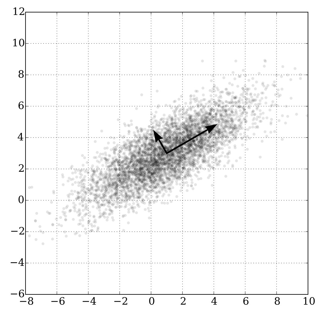
PCA of a multivariate Gaussian distribution
 PCA of a multivariate Gaussian distribution
Source: Wikimedia Commons.

While the data in Figure 1 appears complex, PCA consistently reveals that 95-99% of these movements are driven by just three factors:

1. Level (PC1)

The first component typically explains 80-90% of the variance. It corresponds to a parallel shift in the yield curve: all rates across the surface go up or down together. Traders use this factor to manage Delta or duration risk. When the Federal Reserve raises rates, the entire surface tends to shift upward, in fact this is PC1 in action.

2. Slope (PC2)

The second component explains most of the remaining variance. It corresponds to a tilting of the curve: steepening or flattening. A “curve trade” (e.g., long 2Y, short 10Y) is essentially a bet on this specific principal component.

3. Curvature (PC3)

The third component captures the “butterfly” movement: short and long ends move in one direction, while the belly (medium term) moves in the opposite direction. While it explains little variance (often <2%), it is crucial for pricing convex instruments like swaptions or constructing fly trades (e.g., long 2Y, short 5Y, long 10Y).

Application to Equities: Eigen-Portfolios and Statistical Arbitrage

In equity markets, PCA is used to identify “Eigen-Portfolios”, synthetic portfolios constructed using the eigenvector weights.

The First Principal Component (PC1) almost always represents the Market Mode. Since stocks generally move up and down together, the weights in PC1 are usually all positive. This synthetic portfolio looks very similar to the S&P 500 or a broad market index.

The subsequent components (PC2, PC3, etc.) often represent Sector Modes or other macroeconomic factors (e.g., Oil vs. Tech, or Value vs. Growth). For example, PC2 might be long energy stocks and short technology stocks by capturing the rotation between these sectors.

Quantitative traders use this for Statistical Arbitrage. For example, by regressing a single stock’s returns against the top factors (e.g., the first 5 PCs), they can decompose the return into a “systematic” part (explained by the market) and a “residual” part (idiosyncratic). If the residual deviates significantly from zero, it implies the stock is mispriced relative to its usual correlation structure, traders then buy the stock and hedge the systematic risk using the Eigen-Portfolios, betting that the residual will revert to zero.

Critical limitations of PCA

While being very useful, PCA is not a magic bullet. Quants must be aware of its limitations:

  • 1. PCA only detects linear correlations as it cannot capture complex, non-linear dependencies (like tail dependence during a crash) where correlations tend to spike toward 1.
  • 2. The principal components are statistical constructs, not fundamental laws. They can be unstable over time: what looks like a “Tech factor” today might blend into a “Momentum factor” tomorrow. The eigenvectors can “flip” signs or mix, requiring constant re-estimation.
  • 3. PCA is a “blind” algorithm. It tells you that a factor exists, but not what it is. It is up to the analyst to interpret PC2 as “Slope” or “Inflation Risk.” Without careful interpretation, it can lead to wrong correlations.

Why should I be interested in this post?

For students in Data Science and Finance, PCA is the perfect bridge between machine learning theory and asset management practice. It moves beyond simple diversification (“don’t put all eggs in one basket”) to a mathematical rigor that quantifies exactly how many independent baskets actually exist.

Whether you want to work in Fixed Income (managing curve risk), Equity Derivatives (managing volatility surfaces), or Quantitative Hedge Funds (building neutral alpha signals), PCA is a foundational tool that appears in almost every risk model.

Related posts on the SimTrade blog

   ▶ Youssef LOURAOUI About yield curve calibration

   ▶ Mathias DUMONT Climate-Based Volatility Inputs

   ▶ Youssef LOURAOUI Fama-MacBeth regression method

Useful resources

Statistics

Laloux, L., Cizeau, P., Bouchaud, J. P., & Potters, M. (2000). Random matrix theory and financial correlations. International Journal of Theoretical and Applied Finance, 3(03), 391-397.

d’Aspremont, A., El Ghaoui, L., Jordan, M. I., & Lanckriet, G. R. (2007). A direct formulation for sparse PCA using semidefinite programming. SIAM review, 49(3), 434-448.

Applications in finance

Litterman, R., & Scheinkman, J. (1991). Common factors affecting bond returns, The Journal of Fixed Income, 1(1), 54-61.

Avellaneda, M., & Lee, J. H. (2010). Statistical arbitrage in the US equities market, Quantitative Finance, 10(7), 761-782.

Cont, R., & da Fonseca, J. (2002). Dynamics of implied volatility surfaces, Quantitative Finance, 2(1), 45-60.

About the author

The article was written in December 2025 by Bryan BOISLEVE (CentraleSupélec – ESSEC Business School, Data Science, 2025-2027).

   ▶ Read all articles by Bryan BOISLEVE.
My internship experience as a Counterparty Risk Analyst at Société Générale

Bryan BOISLEVE

In this article, Bryan BOISLEVE (CentraleSupélec – ESSEC Business School, Data Science, 2025-2027) shares his professional experience as a Counterparty Risk Analyst intern within Société Générale’s investment banking division.

About the company

Société Générale is one of the largest European banking groups, offering retail banking, corporate and investment banking, and specialised financial services in over 60 countries. As of 31 December 2024, the Group had around 119,000 employees, served more than 26 million clients in 62 countries, and reported total assets of EUR 1,573.5bn, with total equity of EUR 79.6bn. In 2024, revenues (net banking income) amounted to EUR 26.8bn and group net income (Group share) reached EUR 4.2bn.

Logo of Société Générale
 Logo of Société Générale
Source: the company.

Its Corporate & Investment Banking (CIB) branches serve corporates and institutional investors with financing, capital markets, and risk-management solutions on a diverse range of asset classes (equities, fixed income, derivatives…).

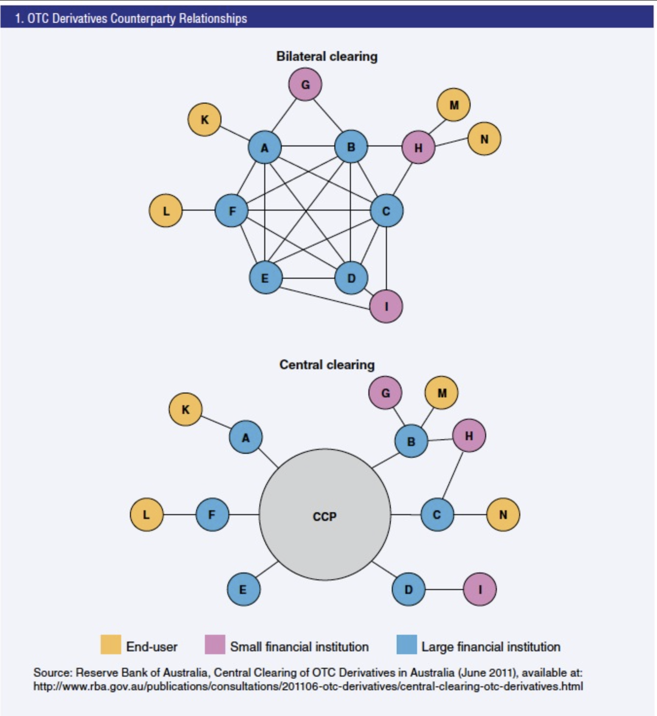
The bank is a major clearing member at leading central counterparties (CCPs), acting as an intermediary between clients and clearing houses for listed and cleared OTC derivatives. This activity is supported by a structured process of daily margining, exposure monitoring, and default fund contributions, embedded within risk management and control functions. The chart below helps illustrate the distribution and scale of OTC derivatives activity, and how a CCP simplifies OTC operations.

Chart of derivatives market structure with CCP
 Chart of derivatives market structure with CCP
Source: Bank Of Australia

During my internship, I worked in the front office counterparty risk team (counterparty risk has also a team in middle office) in Paris, which monitors exposures to central counterparties and major clearing brokers, analyses margin models, and challenges the robustness of CCP risk frameworks used for derivatives clearing.

My internship

Over three months, I focused on cleared derivatives exposures, supporting the team in monitoring house and client portfolios across several CCPs and in assessing whether margin and default fund resources were sufficient under stressed market conditions.

My missions

My main tasks were to analyze house and client risk exposures using Initial Margin (IM), Default Fund (DF), Variation Margin (VM), Value at Risk (VaR) and Conditional VaR (CVaR), to automate DF estimations for two CCPs in Python, to draft annual credit reviews for major central counterparty, and to investigate daily IM and DF breaches together with traders and the wider risk department.

I also implemented an Almgren–Chriss optimal execution model on a client book to better estimate liquidation costs in the Default Management Process, improving the bank’s view on how quickly and at what cost a defaulted portfolio could be unwound.

Required skills and knowledge

This internship required strong quantitative skills (statistics, VaR/CVaR, optimisation), solid understanding of derivatives and CCP mechanics, and programming abilities in Python to automate risk calculations, as well as proficiency with Excel and internal risk systems.

On the soft-skill side, I had to communicate complex risk topics clearly to traders and senior risk managers, work accurately under time pressure when margin breaches occurred, and be proactive in proposing model improvements or new monitoring dashboards.

A good example of how I applied these skills is when my manager asked me to create a dashboard available for key managers that could show the historical exposition and an estimate of this exposition on a specific CCP. After my internship ended, the team decided to implement the model used for the estimation as well as the dashboard for all the CCP where Société Générale was a clearing member.

What I learned

I learned a lot during my internship: how CCPs use margin models, default funds and stress tests to ensure they can withstand the default of major clearing members, and how a bank as a clearing member independently challenges those frameworks to protect its balance sheet.

This experience also taught me to question model assumptions, to combine quantitative analysis with qualitative judgement on CCP governance and transparency, and it confirmed my interest in pursuing a career in quantitative risk management. I also learned how to work with colleage from different countries and different backgrounds which is a soft skills that can really be helpful in a professional environment.

Economic, financial, and business concepts related to my internship

I believe these are three financial concepts related to my internship which are very important: central counterparty default waterfalls, initial margin models, and the Almgren–Chriss optimal execution framework.

Central counterparty default waterfall

The CCP default waterfall is the sequence of financial resources used to absorb losses when a clearing member defaults: the member’s IM, then its DF contribution, then the CCP’s own capital (“skin‑in‑the‑game”), and finally the mutualised default fund and any additional loss-allocation tools.

Understanding this waterfall was crucial in my role, because my analyses assessed whether Société Générale’s exposures and contributions at each CCP were consistent with its risk appetite and with regulatory “Cover‑2” stress-test standards.

Initial margin models (VaR / SPAN)

CCPs typically compute IM with either VaR-based models or SPAN-style scenario approaches, which aim to cover potential losses over a margin period of risk at high confidence levels (often 99% or more).

In my reviews of multiple CCPs, I compared how their IM methodologies capture product risk, concentration risk and wrong-way risk, and how model choices translate into the level and procyclicality of margin calls for the bank and its clients.

Almgren–Chriss optimal execution

The Almgren–Chriss model provides an optimal schedule to liquidate large positions by balancing market impact costs against price risk, typically leading to front‑loaded execution for risk‑averse traders.

By calibrating this model on client portfolios, I helped the team estimate realistic liquidation costs that would arise in a CCP default management auction, improving the calibration of IM add‑ons and internal stress scenarios.

Why should I be interested in this post?

For a student in finance, counterparty risk at a global investment bank like Société Générale, offers a great opportunity on how derivatives markets, CCPs and regulation interact between each other, and shows how quantitative models directly influence daily risk decisions and capital usage.

This type of internship is particularly valuable if you are interested in careers in market risk, XVA, clearing risk or quantitative research, because it combines modelling, coding and discussions with trading desks on real portfolios and real constraints. Overall it is a great internship to have a first step in the trading floor.

Related posts on the SimTrade blog

Profesional experiences

   ▶ All posts about Professional experiences

   ▶ Roberto RESTELLI My internship at Valori Asset Management

   ▶ Julien MAUROY My internship experience as a Finance & Risk Analyst

Financial techniques

   ▶ All posts about Financial techniques

   ▶ Akshit GUPTA Initial and maintenance margins in stocks

   ▶ Akshit GUPTA Initial and maintenance margins in futures contracts

Useful resources

Financial regulation

European Securities and Market Authority (ESMA) Clearing obligation and risk mitigation techniques under EMIR.

Bank of International Settlements (BIS) (April 2012) Principles for financial market infrastructure.

Bank of England (November 2025) Central Counterparty (CCP) policy and rules.

Boudiaf, I., Scheicher, M., Vacirca, F., (April 2023) CCP initial margin models in Europe, Occasional Paper Series, European Central Bank (ECB).

International Swaps and Derivatives Association (ISDA) (August 2013) CCP Loss Allocation at the End of the Waterfall.

Academic research

Almgren, R., Chriss, N., 2000. Optimal execution of portfolio transactions, Working Paper.

Duffie, D., Scheicher, M., Vuillemey, G., 2014. Central Clearing and Collateral Demand, Working Paper.

Pirrong, C., 2013. A Bill of Goods: CCPs and Systemic Risk, Working paper, Bauer College of Business University of Houston.

Berndsen, R., 2021. Fundamental questions on central counterparties: A review of the literature, The Journal of Futures Markets, 41(12) 2009-2022.

About the author

The article was written in December 2025 by Bryan BOISLEVE (CentraleSupélec – ESSEC Business School, Data Science, 2025-2027).

   ▶ Read all articles by Bryan BOISLEVE .