In this article, Bryan BOISLEVE (CentraleSupélec – ESSEC Business School, Data Science, 2025-2027) explores Principal Component Analysis (PCA), a dimensionality reduction technique widely used in quantitative finance to identify the hidden drivers or risk factors of market returns.

Introduction

Financial markets generate large volumes of high-dimensional data, as asset prices and returns evolve continuously over time. For instance, analysing the daily returns of the S&P 500 involves studying 500 distinct but related time series. Treating these series independently is often inefficient, as asset returns exhibit strong cross-sectional correlations driven by common systematic factors (for example: macroeconomic conditions, interest rate movements, and sector-specific shocks).

This why we have the Principal Component Analysis (PCA) which is a powerful statistical method used to simplify this complexity. It transforms a large set of correlated variables into a smaller set of uncorrelated variables called Principal Components (PCs). By retaining only the most significant components, quants can filter out the “noise” of individual stock movements and isolate the “signal” of broad market drivers.

The Mathematics: Eigenvectors and Eigenvalues

PCA is an application of linear algebra to the covariance (or correlation) matrix of asset returns. The goal is to find a new coordinate system that best preserves the variance of the data.

If we have a matrix X of standardized returns (where each asset has a mean of 0 and variance of 1), we compute the correlation matrix C. We then perform an eigendecomposition:

Cv = λv

• Eigenvectors (v) define the direction of the principal components. In finance, these vectors act as “weights” for constructing synthetic portfolios.
• Eigenvalues (λ) represent the magnitude of variance explained by each component. The ratio \( \lambda_i / \sum \lambda \) tells us the percentage of total market risk explained by the i-th component.

A key property of PCA is orthogonality: the resulting principal components are mathematically uncorrelated with each other. This is very useful for risk modeling, as we can sum up the variances of individual components to estimate total portfolio risk without worrying about cross-correlations.

Classic Application: Decomposing the Yield Curve

The most famous application of PCA in finance is in Fixed Income markets. A yield curve consists of interest rates at many maturities (1M, 2Y, 5Y, 10Y, 30Y). As shown in the image below, the history of US yield curves forms a complex “surface” that evolves over time.

Figure 1. PCA of a multivariate Gaussian distribution

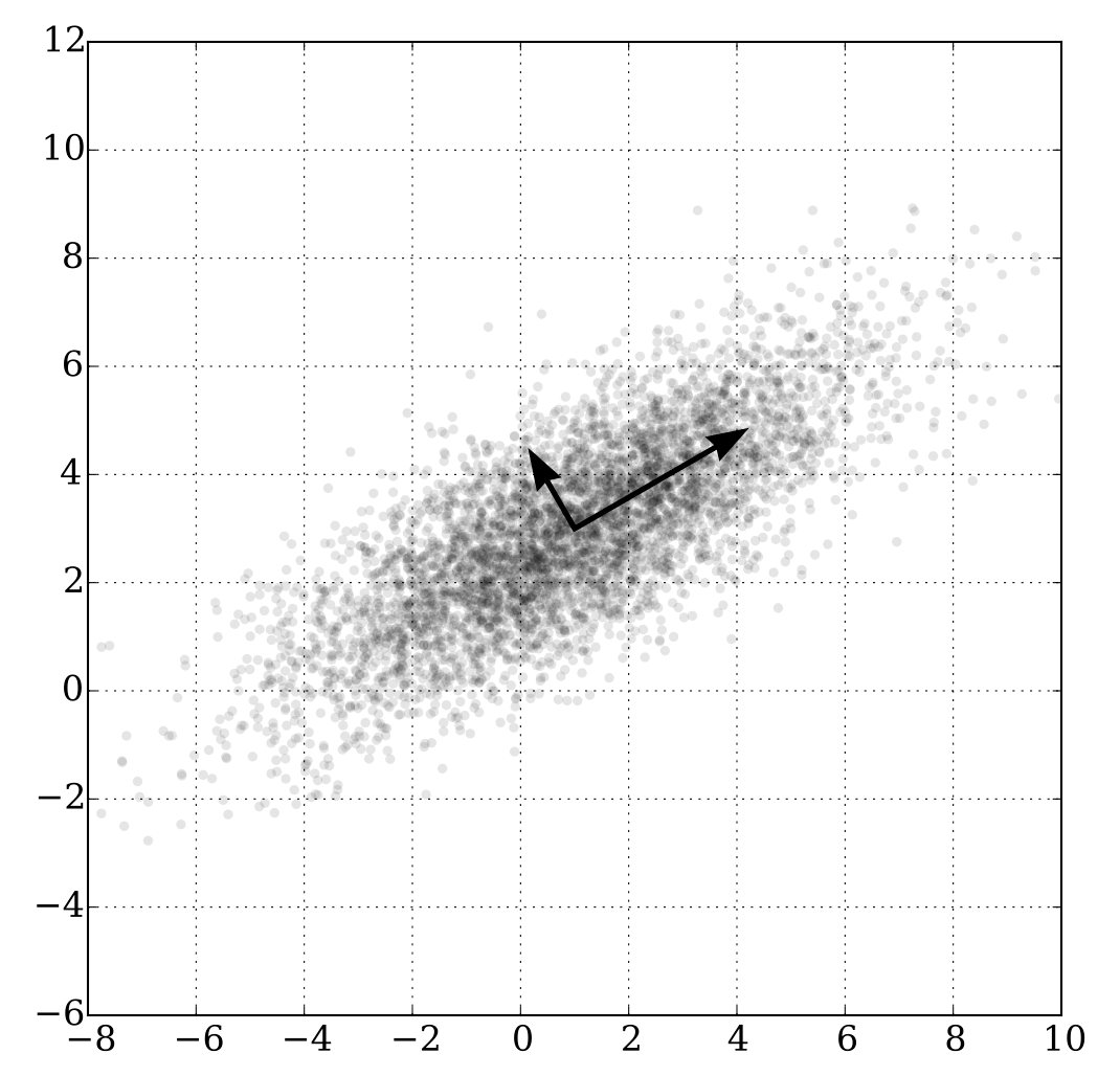
Source: Wikimedia Commons.

While the data in Figure 1 appears complex, PCA consistently reveals that 95-99% of these movements are driven by just three factors:

1. Level (PC1)

The first component typically explains 80-90% of the variance. It corresponds to a parallel shift in the yield curve: all rates across the surface go up or down together. Traders use this factor to manage Delta or duration risk. When the Federal Reserve raises rates, the entire surface tends to shift upward, in fact this is PC1 in action.

2. Slope (PC2)

The second component explains most of the remaining variance. It corresponds to a tilting of the curve: steepening or flattening. A “curve trade” (e.g., long 2Y, short 10Y) is essentially a bet on this specific principal component.

3. Curvature (PC3)

The third component captures the “butterfly” movement: short and long ends move in one direction, while the belly (medium term) moves in the opposite direction. While it explains little variance (often <2%), it is crucial for pricing convex instruments like swaptions or constructing fly trades (e.g., long 2Y, short 5Y, long 10Y).

Application to Equities: Eigen-Portfolios and Statistical Arbitrage

In equity markets, PCA is used to identify “Eigen-Portfolios”, synthetic portfolios constructed using the eigenvector weights.

The First Principal Component (PC1) almost always represents the Market Mode. Since stocks generally move up and down together, the weights in PC1 are usually all positive. This synthetic portfolio looks very similar to the S&P 500 or a broad market index.

The subsequent components (PC2, PC3, etc.) often represent Sector Modes or other macroeconomic factors (e.g., Oil vs. Tech, or Value vs. Growth). For example, PC2 might be long energy stocks and short technology stocks by capturing the rotation between these sectors.

Quantitative traders use this for Statistical Arbitrage. For example, by regressing a single stock’s returns against the top factors (e.g., the first 5 PCs), they can decompose the return into a “systematic” part (explained by the market) and a “residual” part (idiosyncratic). If the residual deviates significantly from zero, it implies the stock is mispriced relative to its usual correlation structure, traders then buy the stock and hedge the systematic risk using the Eigen-Portfolios, betting that the residual will revert to zero.

Critical limitations of PCA

While being very useful, PCA is not a magic bullet. Quants must be aware of its limitations:

• 1. PCA only detects linear correlations as it cannot capture complex, non-linear dependencies (like tail dependence during a crash) where correlations tend to spike toward 1.
• 2. The principal components are statistical constructs, not fundamental laws. They can be unstable over time: what looks like a “Tech factor” today might blend into a “Momentum factor” tomorrow. The eigenvectors can “flip” signs or mix, requiring constant re-estimation.
• 3. PCA is a “blind” algorithm. It tells you that a factor exists, but not what it is. It is up to the analyst to interpret PC2 as “Slope” or “Inflation Risk.” Without careful interpretation, it can lead to wrong correlations.

Why should I be interested in this post?

For students in Data Science and Finance, PCA is the perfect bridge between machine learning theory and asset management practice. It moves beyond simple diversification (“don’t put all eggs in one basket”) to a mathematical rigor that quantifies exactly how many independent baskets actually exist.

Whether you want to work in Fixed Income (managing curve risk), Equity Derivatives (managing volatility surfaces), or Quantitative Hedge Funds (building neutral alpha signals), PCA is a foundational tool that appears in almost every risk model.

Related posts on the SimTrade blog

   ▶ Youssef LOURAOUI About yield curve calibration

   ▶ Mathias DUMONT Climate-Based Volatility Inputs

   ▶ Youssef LOURAOUI Fama-MacBeth regression method

Useful resources

Statistics

Laloux, L., Cizeau, P., Bouchaud, J.P., and Potters, M. (2000). Random matrix theory and financial correlations, International Journal of Theoretical and Applied Finance, 3(03), 391-397.

d’Aspremont, A., El Ghaoui, L., Jordan, M. I., and Lanckriet, G. R. (2007). A direct formulation for sparse PCA using semidefinite programming, SIAM review, 49(3), 434-448.

Applications in finance

Litterman, R., & Scheinkman, J. (1991). Common factors affecting bond returns, The Journal of Fixed Income, 1(1), 54-61.

Avellaneda, M., & Lee, J. H. (2010). Statistical arbitrage in the US equities market, Quantitative Finance, 10(7), 761-782.

Cont, R., & da Fonseca, J. (2002). Dynamics of implied volatility surfaces, Quantitative Finance, 2(1), 45-60.

Python code

Bryan Boislève Principal Component Analysis (PCA) on S&P 500 Sector ETFs (Python code)

About the author

The article was written in December 2025 by Bryan BOISLEVE (CentraleSupélec – ESSEC Business School, Data Science, 2025-2027).

   ▶ Read all articles by Bryan BOISLEVE.