In this article, Cornelius HEINTZE (ESSEC Business School, Global Bachelor in Business Administration (GBBA) – Exchange Student, 2025) explains how the two-stage valuation model and the segmentation in growth stage and stable phase impact the valuation of companies and which problems tend to arise with the use of this model.
Why this is important
The valuation of companies is always present in the world of finance. We see it in Mergers and Acquisitions (M&A), initial public offerings (IPOs) and daily stock market pricing where firms are valued within seconds based on new information. For markets to function properly, valuations need to represent the underlying company as precisely as possible. Otherwise, information asymmetries increase, leading to inefficient or even dysfunctional markets.
The Two-Stage Model
The Two-Stage Model is the traditional model that is used by finance experts across the world. What makes it stand out is the segmentation of the valuation in two steps:
- Growth phase (explicit forecast period):
In this phase, the company’s future cash flows are projected in detail for each year t = 1 … T.
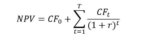
These cash flows are then discounted back to the valuation date using the discount rate r:
PV(Growth phase) = Σt=1…T ( CFt ) / (1 + r)t - Stable phase (terminal value):
After the explicit forecast horizon, the company is assumed to enter a stable stage. There are two assumptions needed to fulfill this stage and its equations. First it is assumed that the company can realize the cashflows over an indefinite timespan. Second, it is assumed that the perpetual growth rate g does not exceed the growth rate of the whole economy. The two common resulting equations are:
- No growth (steady state):
PV(Stable phase) = CFstable / (r * (1 + r)T) - Constant growth in perpetuity:
PV(Stable phase) = CFT+1 / ((r − g) * (1 + r)T)
- No growth (steady state):
Total firm value is then the sum of both parts:
Value = PV(Growth phase) + PV(Stable phase)
Problems with the Two-Stage Model
If we look closer at the equations for the stable phase you will realize that they show a perpetuity. Looking at the assumptions given, this is also the only possible outcome. But given this circumstance we encounter the first big problem of the Two-Stage Model: the stable phase often makes up over 50% of the firm value. This is a problem as the assumptions for the stable phase are often very subjective and not very realistic. The problem evolves even more when it is assumed that there is a constant growth rate. Let’s look at this through an example:
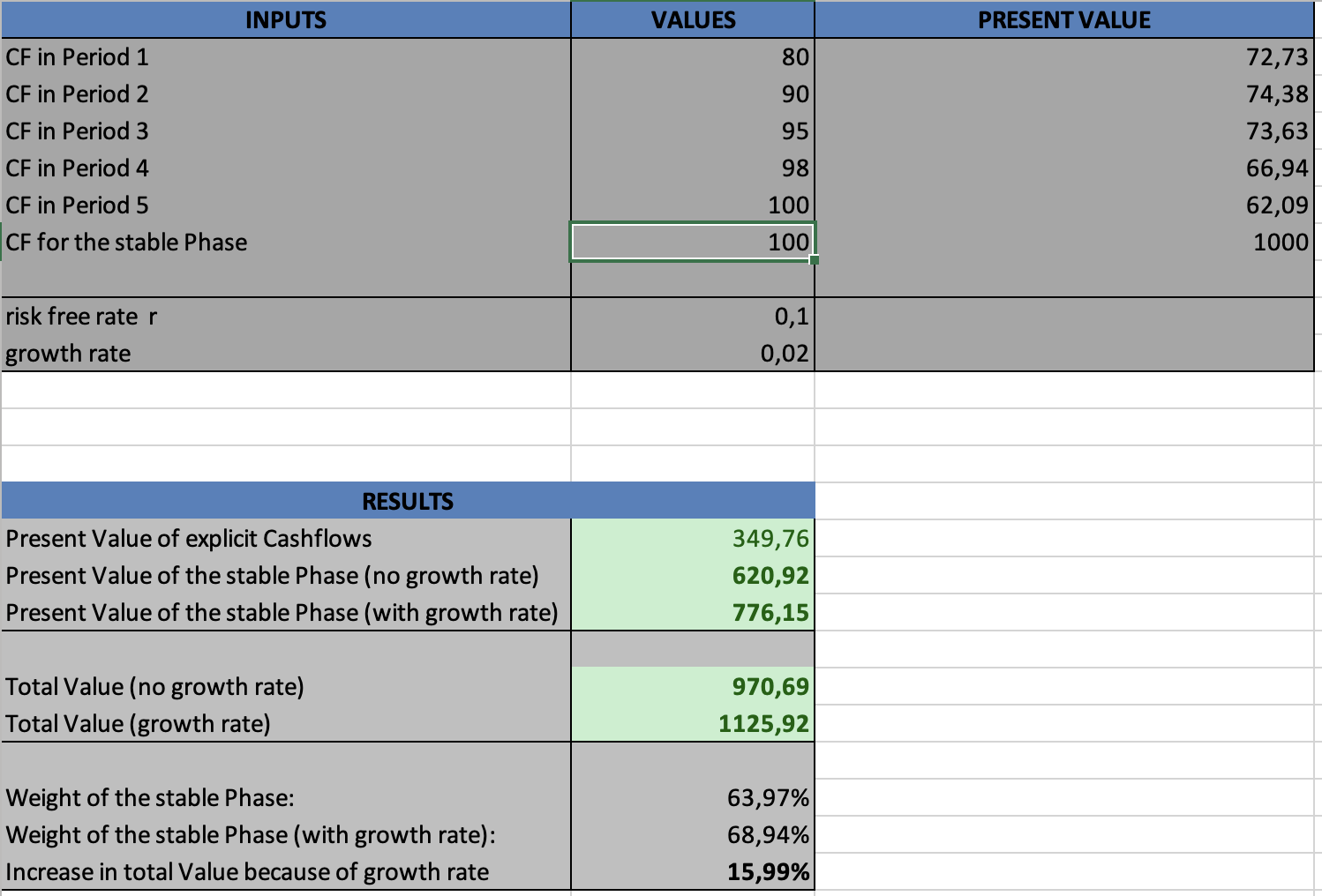
Assumptions: discount rate r = 10%, explicit forecast over T = 5 years with free cash flows (in €m): 80, 90, 95, 98, 100. After year 5, we consider two terminal cases.
Phase 1 – Present value of explicit cash flows
- Year 1: 80 / (1.10)1 = 72.73
- Year 2: 90 / (1.10)2 = 74.38
- Year 3: 95 / (1.10)3 = 71.37
- Year 4: 98 / (1.10)4 = 66.94
- Year 5: 100 / (1.10)5 = 62.09
PV(Phase 1) ≈ 347.51 (€m)
Phase 2 – Stable phase
- (a) No growth: CFstable = 100 ⇒ TV at t=5
PV(Terminal) = 100 /(0.1*(1.10)5) = 620.92 - (b) Constant growth g = 2%: CFT+1 = 100 ⇒ TV at t=5
PV(Terminal) = 100/((0.10-0.08) * (1.10)5) = 776.15
Total value and weights
- No growth: Total = 347.51 + 620.92 = 968.43 ⇒ Stable Phase share ≈ 64.1%, Phase-1 share ≈ 35.9%
- g = 2%: Total = 347.51 + 776.15 = 1,123.66 ⇒ Stable Phase share ≈ 69.1%, Phase-1 share ≈ 30.9%
- Impact of growth: Increase in the firm value of 155.23 or ≈ 16%
Takeaway: A modest increase in the perpetual growth rate from 0% to 2% raises the terminal present value by ~155 (€m) and lifts its weight from ~64% to ~69% of total value. This illustrates the strong sensitivity of the two-stage model to terminal assumptions.
If you want to try out for yourself and learn more about the sensitivity of the growth rate in relation to the firm value you can do so in the excel-file I have created in order for this example as shown below:
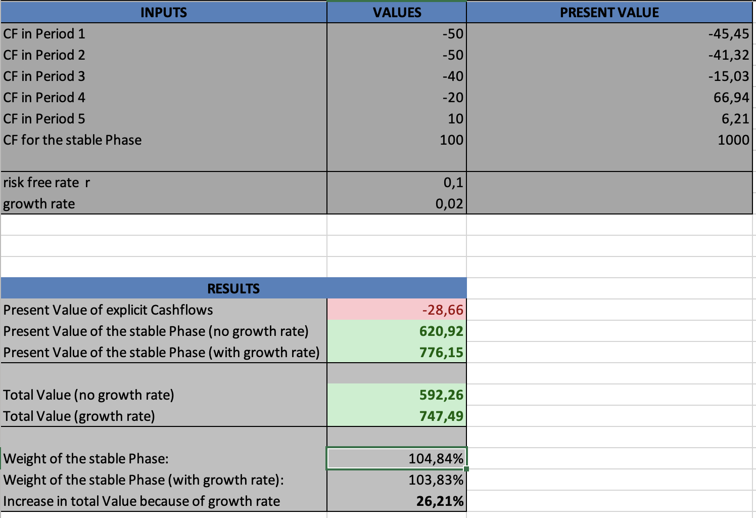
Another very interesting fact gets visible, while trying out the model, which is commonly seen in early tech startups or general startups, that have very high early investment costs (for example software development). They will have a negative firm value in the growth phase but in the long run it is assumed that these companies will have a constant growth rate and positive cashflows, therefore evening out the negative growth phase. This again shows how much of an impact the stable and the growth phase has on the firm value.
You can download the excel file here:

Implications for practical use and solutions
As seen in the example, the impact of the stable phase and therefore the assumptions about the cashflows and the circumstances of the company as to whether it is appropriate to use a growth rate plays a big role in on the valuation of the firm. Deciding these assumptions lies at the feet of the firms that valuate the company or at the company valuating itself. Therefore, they are highly subjective and must be transparent at all times to ensure an appropriate valuation of the firm. If this is not the case firms can be valued at a much higher value than it is appropriate and therefore convey false information.
To fight this it is recommended to incorporate various valuation methods to verify that the value is not too high or too low but rather on a bandwidth of values which are plausible. This is often times part of a fairness opinion which is issued by an independent company. You can see an example here when Morgan Stanley drafted a fairness opinion for Monsanto for the merger with Bayer:
Full SEC Statement for the merger
To sum up…
The Two-Stage Valuation Model remains a cornerstone in corporate finance because of its simplicity and structured approach. However, as the example shows, the stable phase dominates the overall result and makes valuation highly sensitive to small changes in assumptions. In practice, analysts and other users of the information provided by the valuing company should therefore apply the model with caution, test alternative scenarios, and complement it with other methods. Looking ahead, the combination of traditional models with advanced techniques such as multi-stage models, sensitivity analyses, or even simulation approaches can provide a more balanced and reliable picture of a company’s value.
Why should I be interested in this post?
Whether you are a student of finance, an investor, or simply curious about how firms are valued, understanding the Two-Stage Valuation Model is essential. It is one of the most widely used approaches in practice and often determines the prices we see in the markets, from IPOs to M&A. By being aware of both its strengths and its limitations, you can better interpret valuation results and make more informed financial decisions.
Related posts on the SimTrade blog
▶ All posts about financial techniques
▶ Jorge KARAM DIB Multiples valuation methods
▶ Andrea ALOSCARI Valuation methods
▶ Samuel BRAL Valuing the Delisting of Best World International Using DCF Modeling
Useful resources
Paul Pignataro (2022) “Financial modeling and valuation: a practical guide to investment banking and private equity” Wiley, Second edition.
Tim Koller, Marc Goedhart, David Wessels (2010) “Valuation: Measuring and Managing the Value of Companies”, McKinsey and Company.
About the author
The article was written in October 2025 by Cornelius HEINTZE (ESSEC Business School, Global Bachelor in Business Administration (GBBA) – Exchange Student, 2025